Numba is an Python Just In Time compiler that essentially translates Python functions into fast machine code using LLVM. With the relatively recent boom of data-driven programming, Numba’s library is gaining more attention from its developers and community. (Sponsored by NVidia, Anaconda, Inc., DARPA, Intel…)
In the documentation, Numba advertises JIT performace similar to C, C++, and Fortran!
Numba’s motto is to keep things simple. You shouldn’t have to spend hours optimizing code when the opportunity cost isn’t worth it. In many cases, Numba has the benefit of massively accelerating your computing with little code modification. If the following describes your code, Numba can help you out:
Prescription drug ad disclaimer: Numba can speed these up [but keep Numba’s limitations in mind (see “Limitations to be aware of” section for more details)]
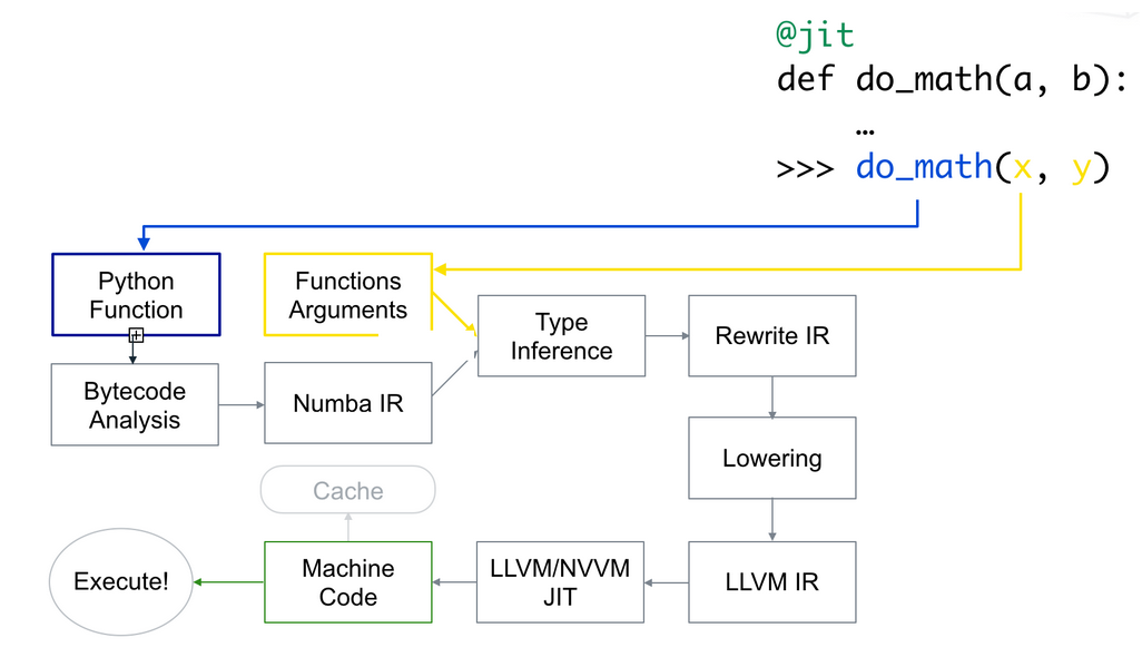
Let’s see what’s going on under the hood…
When you add the @jit decorator, Numba analyzes the Python bytecode and translates it to Numba IR (think of this as Numba’s own bytecode) which is “lowered” to a low-level, machine specific language using the LLVM compiler (think Assembly). Then by passing cache=True, this is also True by default, you can instruct Numba to write the resulting compilation into a cache, which avoids compilation time on the next run.
You can instruct Numba to compile your function independent of the Python interpreter. In fact, this is considered “best practice” as it leads to the best performace.
You can tell Numba to execute No Python mode in two ways:
@jit(nopython=True)
or its alias:
@njit
However, you need to use from njit import numba for the latter.
If Numba comes across Python code it cannot understand, it falls back to “Object Mode”. For instance, as of Numba 0.51.2, dictionaries are not supported. If you try to compile a function with a dictionary with @jit, you may be surprised to see that Numba was still able to compile the function since it uses Object mode to enable other Numba functionality.
But given what was just said, in many cases, you can tell Numba provide information when type interface fails by passing nopython=True into the decorator argument. In this case, you will come across the error:
- argument 0: cannot determine Numba type of <class 'dict'>
@vectorizeTo optimize a ufunc with Numba, decorate the function with @vectorize. This will instruct Numba to parallelize the function that is decorated. Some arguments will need to be passed in order to process the function on the GPU.
When working with Numpy arrays, another benefit to using Numba is that it will figure out broadcasting rules for different arrays with compatible dimensions.
The first time you throw @jit on top of you function, you will find that your function actually take longer to run. Why?
Since Numba is a JIT compiler, when you run the function, Numba will compile the code using LLVM for the first run, introducing some overhead. Once the code is cached and ran a second time, it will result in an optimized run time.
There is work to support as much of the Python language as possible but some widely used features are not available in Numba compiled functions:
dict/list/exception/set are partially supported (usually means you have to use an alternative e.g. typed lists)
mixing types confuses Numba
Some popular libraries are partially supported(p)/not supported(n):
%timeitWhen benchmarking Numba code, it would be best to use %timeit which runs a function or loop multiple times to accurately get an estimate of run time. The output is the mean and standard deviation of multiple runs. Hence, accomodating for the compilation time of the first execution.
NumPy arrays operate element-wise. NumPy ufuncs or “universal functions” operate in the same fashion. For instance, np.sin(a) applies \(sin\) to each element in array a . For example,
a = [1,2,3,4]
np.sin(a)
Output:
array([ 0.84147098, 0.90929743, 0.14112001, -0.7568025 ])
Indexing arrays is pretty straight forward (at least for me, it’s easier to think in terms of rows). However, slicing can get very interesting, very quickly. Slicing syntax is as follows:
var[lower:upper:step]
Consider the array,
var = np.array([7,8,9,10,11,12])
Some examples of omitting indicies in the array:
Choosing the first 3 elements
var[:3]
Output:
array([7, 8, 9])
Choosing the last two elements
var[-2:]
Output:
array([11,12])
Choosing every other element
var[::2]
Output:
array([ 7, 9, 11])
Consider a \(4 \times 5\) 2-D array called two_d:
array([[ 0,  1,  2,  3,  4],
       [ 5,  6,  7,  8,  9],
       [10, 11, 12, 13, 14],
       [15, 16, 17, 18, 19]])
We can choose the 3rd column by using the “lonely colon”,
choose3rdcol = two_d[:,2]
choose3rdcol
Output:
array([ 2, 7, 12, 17])
Row selection works the same way,
choose2ndrow = two_d[1,:]
choose2ndrow
Output:
array([5, 6, 7, 8, 9])
However, keep in mind that these outputs for row/column selection are 1-D arrays. In other words, the column selected output is a row of the column elements.
if __name__ = __main__Colloquially, when this shows up in python code, this signals to those who are reading it that this particular file is running as a script.
Lambdas in python are “anonymous functions”, in that they do not occupy a namespace. In other words, Lambdas are equivalent to the standard input-output function, which is function declarations:
def add_one(x):
    return x + 1
The advantage of using lambda is that you can define the same function inline. Since Lambdas are not “named”, they are function expressions:
a = lambda x: x + 1
To evaluate the function:
print(a(1))
yields:
2