\(\let\vec\mathbf\) \(\newcommand{\v}{\vec}\) \(\newcommand{\d}{\dot{}}\) \(\newcommand{\del}{\nabla}\) \(\newcommand{\abs}{\rvert}\) \(\newcommand{\h}{\hat}\) \(\newcommand{\f}{\frac}\) \(\newcommand{\~}{\widetilde}\) \(\newcommand{\<}{\langle}\) \(\newcommand{\>}{\rangle}\) \(\newcommand{\eo}{\epsilon_{0}}\) \(\newcommand{\hb}{\hbar}\) \(\newcommand{\pd}{\partial}\) \(\newcommand{\h}{\hat}\) \(\newcommand{\ket}[1]{\lvert #1 \rangle}\)
The state of a quantum mechanical system is described by a wavefunction \(\Psi(\v{r},t)\), which is mathematically interpreted as a state vector \(\ket{\Psi}\) that belongs to a state space called the Hilbert space and is a function of position \(\v{r}\) and time \(t\). For an isolated system, the probability of finding the particle somewhere must be equal to one.
\[\int_{-\infty}^{+\infty} \Psi^{*}(\v{r},t) \Psi(\v{r},t) d\tau = 1\]The term \(\Psi^{*}(\v{r},t) \Psi(\v{r},t) d\tau\) defines the probability of finding the particle in volume \(d\tau\) at \(\v{r}\) and \(t\).
Physical observables are represented as operators in quantum mechanics. Operators have the property of being linear and Hermitian. In other words, a physical quantity \(A\) is described by a Hermitian operator \(\h{A}\) acting in state space \(H\), forming a basis for \(H\). The result of measuring \(A\) results in
The wavefunction or state function evolves in time according to the time independent Schrodinger equation:
\[i\hbar \f{\pd \Psi}{\pd t} = \h{H} \Psi\]For a given potential energy function \(V(x,t)\), the Schrodinger equation, independent of \(t\) is written as:
\[i \hb \f{\pd \Psi}{\pd t} = - \f{\hb^{2}}{2m} \f{\pd^{2} \Psi}{\pd x^{2} } + V \Psi\]Consider a situation where a particle is trapped in a potential well with infinitely high walls. The potential is described mathematically as,
\[V(x) = \left\{ \begin{array}{ll} 0 & 0 \leq x \leq a, \\ \infty & \verb|otherwise| \\ \end{array} \right.\]The time indpendent Schrodinger equation can be set up using known conditions of the system.
Outside the well, the probability of finding the particle equal to zero, in other words, the wavefunction is \(\Psi(x) = 0\).
Inside the well, the potential is \(V=0\)
The Schrodinger equation then takes the form,
\[- \f{\hb^{2}}{2m} \f{d^{2} \psi}{dx^{2}} = E \psi\]We can divide through by \(-\f{\hb^{2}}{2m}\) and where \(k \equiv \f{\sqrt{2mE}}{\hb}\)
\[\f{d^{2} \psi}{dx^{2}} = - k^{2} \psi\]The general solution this differential equation is,
\[\psi(x) = A\sin{kx} + B\cos{kx}\]With both the wave function, \(\psi\), and its derivative ,\(\f{d\psi}{dx}\), being continuous, this just means that both are differentiable.
Applying the boundary conditions, the continuity of \(\psi(x)\) require that
\[\psi(0) = \psi(a) = 0\]Thus at \(\psi(0)\),
\[\psi(0) = 0 = A \sin{0} + B\cos{0} = B\]Plugging \(B = 0\) back into the general solution yields
\[\psi(x) = A \sin{kx}\]At \(\psi(a)\), we come across two cases in order to satify \(\psi(a) = 0\). The wavefunction at \(a\) is,
\[\psi(a) = A \sin{ka}\]The two cases being,
\(A=0\), non-normalizable \(\psi(x) = 0\) (not a good solution, the wavefunction MUST appear somewhere!)
\(\sin{ka} = 0\), which allows the existence of \(\psi\)
The latter is only true for certain values of \(ka\),
\[ka = 0, \pm \pi, \pm 2\pi, \pm 3\pi, ...\]Again, we come across another “bad” solution, \(k = 0\), since this would imply that \(\psi(x) = 0\). The minus sign from negative solutions such as \(\sin(-\theta) = -\sin(\theta)\) can be absorbed into the constant \(A\).
Thus, we arrive at distinct solutions where,
\[k_{n} = \f{n\pi}{a}\]with values of \(n = 1, 2, 3, ...\). Combining this with definition of \(k\) in terms of energy \(E\),
\[E_{n} = \f{\hbar^{2} k_{n}^{2}}{2m} = \f{n^{2} \pi^{2} \hb^{2}}{2ma^{2}}\]To interpret this physically, the energy \(E_{n}\) can only take on discrete values of \(n\). We also attach the subscript \(n\) to denote that \(k_{n}\) represents the set of allowed energies of the wavefunction, which will be important to evaluating the upcoming integral.
However, \(A\) is still a missing part of the equation, which is determined by \(k\). We can solve for \(A\) by normalizing \(\psi\).
\[\int_{0}^{a} \abs A \abs^{2} \sin^{2}(k_{n} x) dx = \abs A \abs^{2} \int_{0}^{a} \f{1- \cos(2k_{n} x)}{2} dx = 1\]With the help of a trigonometric identity: \(\sin^{2} (\theta) = \f{1-\cos(2\theta)}{2}\)…
Using u-subsitution, let \(u=2k_{n} x\), where \(du = 2k_{n} dx\),
\[\abs A \abs^{2} \bigg[ \f{x}{2} \bigg|_{0}^{a} - \int_{0}^{a} \f{\cos{u}}{2} \f{du}{2} \bigg] = 1\] \[\abs A \abs^{2} \bigg[ \f{x}{2} - \f{\sin{2k_{n} x}}{4k} \bigg]_{0}^{a} = 1\]Now it is important to recall that \(k= \f{n \pi}{a}\). \(k\) is restricted by \(n = 1,2,3,...\) and for this reason, the \(\sin2kx\) term is zero at all values of \(n\). Now simply solving for \(A\) will yield the magnitude of \(A\), picking the positive solution.
\[\abs A \abs^{2} \f{a}{2} = 1\] \[A = \sqrt{\f{2}{a}}\]Thus, the wavefunction solutions inside the well is,
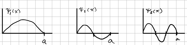
\[\psi_{n} (x) = \sqrt{\f{2}{a}} \sin\bigg(\f{n\pi x}{a}\bigg)\]
Note that the solutions alternate between even and odd between the intervals [0, a] . \(\psi_{1}\) is even, \(\psi_{2}\) is odd, \(\psi_{3}\) is even. This also related to how many nodes, or zero crossings, for successive states \(\psi_{n}\). The wave function that carries the lowest energy ,\(n=1\), is the ground state, whereas wavefunctions of energies proportional to \(n^{3}\) are the excited states.
Due to the \(\sin\) terms in states \(\psi_{n} (x)\) end up being mutually orthogonal. In other words,
\[\int \psi_{m} (x)^{*} \psi_{n}(x) dx = 0\]when \(m \neq n\).
\[\int \psi_{m} (x)^{*} \psi_{n}(x) dx = \f{2}{a} \int_{0}^{a} \sin{\bigg( \f{m\pi x}{a} \bigg)} \sin{\bigg( \f{n\pi x}{a} \bigg)} dx\]Orthogonality:
Using a product-to-sum trigonometric identity: \(\sin(\alpha)\sin(\beta) = \f{1}{2} [\cos(\alpha - \beta) - \cos(\alpha + \beta)\)
\(= \f{1}{a} \int_{0}^{a} \cos{\bigg(\f{ (m-n) \pi }{a} \bigg)} - \cos{\bigg(\f{ (m+n) \pi }{a} \bigg)} dx\) \(= \f{1}{a} \bigg[ \f{1}{ (m-n) \pi } \sin{\bigg(\f{ (m-n) \pi }{a} \bigg)} - \f{1}{(m+n) \pi} \sin{\bigg(\f{ (m+n) \pi }{a} \bigg)} \bigg] \bigg|_{0}^{a}\)
When evaluating from \(0\) to \(a\), it should be clear to see that only \(a\) survives, leaving
\(= \f{1}{\pi} \bigg[ \f{ \sin{\bigg(\f{ (m-n) \pi }{a} \bigg)}}{(m-n)} - \f{\sin{\bigg(\f{ (m+n) \pi }{a} \bigg)}}{(m+n)} \bigg] = 0\) (for \(m\neq n\))
Rewritten in terms of the Kronecker Delta,
\[\int \psi_{m} (x)^{*} \psi_{n}(x) dx = \delta_{mn}\]
Consider an electron in a vacuum, without any external influences (i.e. electromagnetic fields). The linear momentum operator is:
\[- i \hbar \nabla \psi = \v{p} \psi\]with \(\v{p}\) being the associated eigenvalues. The wavefunction of an electron in a vacuum is:
\[\psi = e^{i(\v{k}\cdot \v{r} - \omega t)}\]Expanding \(\v{k}\), \(\v{r}\), and \(\nabla\) into their linear components gives,
\[- i \hbar \bigg( \f{\pd{}}{\pd{x}} \h{i} + \f{\pd{}}{\pd{y}} \h{j} + \f{\pd{}}{\pd{z}} \h{k} \bigg) e^{i (k_{x}x + k_{y} y + k_{z} z)} = \v{p} e^{i(\v{k} \cdot {r} - \omega t)}\]The momentum operator acting on \(\psi\) demonstrates that the eigenvalue \(\v{p}\) is,
\[\v{p} = \hbar \bigg( k_{x} \h{i} + k_{y} \h{j} + k_{z} \h{k} \bigg) = \hbar \v{k}\]Using some basic equations from wave mechanics,
\[\lambda = \f{h}{p}\] \[k = | \v{k} | = \f{2\pi}{\lambda}\]It shows that,
\[p = \hbar k = \bigg(\f{h}{2\pi} \bigg) \bigg(\f{2\pi}{\lambda} \bigg)\]Many of the following derivations are rooted in the continuity equation,
\[\frac{\pd \rho_{P}}{\pd t} + \del \cdot \v{J}_{P} = 0\] \[\frac{\pd \rho_{M}}{\pd t} + \del \v{J}_{M} = 0\] \[\frac{\pd \rho_{E}}{\pd t} + \del \v{J}_{E} = 0\]where \(P\), \(M\), and \(E\) represent probability, momentum, and energy currents.
Before deriving flux quantities, it will be useful to mention the following relationships and identities:
\[\frac{\pd \psi}{\pd t} = \f{1}{i\hbar} \bigg[ -\f{\hbar^{2}}{2m} \del^{2} \psi + V \psi \bigg]\]The complex conjugate of \(\frac{\pd \psi}{\pd t}\) is simply,
\[\frac{\pd \psi^{*}}{\pd t} = \f{1}{i\hbar} \bigg[ -\f{\hbar^{2}}{2m} \del^{2} \psi^{*} + V \psi^{*} \bigg]\]Moreover, the two operator identities that will be of use,
\[\del \cdot (\psi^{*} \del \psi) = \del \psi^{*} \cdot \del \psi - \psi^{*} \cdot \del^{2} \psi\] \[\del \cdot (\psi \del\psi^{*}) = \del \psi \cdot \del \psi^{*} - \psi \cdot \del^{2} \psi^{*}\]Lastly, we define the “density”, \(\rho\), with units of “amount per unit volume” as,
\[\rho = \psi^{*} \psi\]The probability density given as,
\[\rho_{P} (\v{r}, t) = \psi^{*}(\v{r},t) \psi(\v{r},t)\]take the partial with respect to time,
\[\f{\pd \rho_{P}}{\pd t} = \bigg( \f{\pd \psi^{*}}{\pd t} \bigg) \psi + \psi^{*} \bigg( \f{\pd \psi }{\pd t} \bigg)\]we plug the expressions of \(\f{\pd \psi}{\pd t}\) and its complex conjugate defined above into the equation,
\[\f{\pd \rho_{P}}{\pd t} = \f{\pd \psi^{*}\psi}{\pd t} = \f{1}{i\hbar} \bigg[ -\f{\hbar^{2}}{2m} \del^{2} \psi^{*} + V \psi^{*} \bigg] \psi + \f{1}{i\hbar} \bigg[ -\f{\hbar^{2}}{2m} \del^{2} \psi + V \psi \bigg] \psi^{*}\] \[= -\f{\hbar}{2mi} (\del^{2} \psi) \psi^{*} + V \psi \psi^{*} + \f{\hbar}{2mi} (\del^{2} \psi^{*} ) \psi - V \psi^{*} \psi\] \[= -\f{\hbar}{2mi} \bigg( (\del^{2} \psi )\psi^{*} + (\del^{2} \psi^{*} )\psi \bigg)\] \[\f{\pd \rho_{P}}{\pd t} = -\f{\hbar}{2mi} \del \bigg( (\del \psi )\psi^{*} + (\del \psi^{*} )\psi \bigg)\]Now that we have an expression for \(\f{\pd \rho_{P}}{\pd t}\), we can apply the continuity equation, which is also a statement of conservation,
\[\f{\pd \rho_{P}}{\pd t} + \f{\hbar}{2mi} \del \bigg( (\del \psi )\psi^{*} + (\del \psi^{*} )\psi \bigg) = 0\]Thus, the second term in the right hand side of the equation tells us that the probability current is,
\[\v{J}_{P} = \f{\hbar}{2mi} \bigg( (\del \psi )\psi^{*} + (\del \psi^{*} )\psi \bigg)\]In a similiar fashion, we can also derive the “momentum current”, \(j_{M}\), given a momentum density,
\[\rho_{M} (\v{r}, t) = \Re{ (\psi^{*} (\v{r},t) \h{p} \psi(\v{r},t) )}\]Again, we take the partial derivative with respect to time,
\[\f{\pd \rho_{M}}{\pd t} = \bigg( \f{\pd \psi^{*}}{\pd t} \bigg) \h{p} \psi + \psi^{*} \h{p} \bigg( \f{\pd \psi }{\pd t} \bigg)\]where the momentum operator is \(\h{p} = -i \hbar \del\).
We substitute the definitions of \(\f{\pd \psi^{*}}{\pd t}\) and \(\f{\pd \psi}{\pd t}\) from above. Keep in mind that we are only considering the real component of the entire expression (the momentum operator happens to be complex).
\[= \Re \biggl\{ \f{1}{i\hbar} \bigg[-\f{\hbar^{2}}{2m} \del^{2} \psi^{*} \h{p} \psi + V \psi^{*} \h{p} \psi \bigg] \biggr\} + \Re \biggl\{ \f{1}{i\hbar} \bigg[ -\f{\hbar^{2}}{2m} \psi^{*} \h{p} \del^{2} \psi + \psi^{*} \h{p} V \psi \bigg] \biggr\}\]substituting the definition of the momentum operator,
\[\f{\pd \rho_{M}}{\pd t} = \Re \biggl\{ \f{\hbar^{2}}{2m} \del^{2} \psi^{*} \del \psi - i\hbar V \psi^{*} \del \psi + \f{\hbar^{2}}{2m} \psi^{*} \del(\del^{2} \psi) - i\hbar \psi^{*} \del V \psi \biggr\}\]and grouping terms involving potential together,
\[= \Re \biggl\{ \f{\hbar^{2}}{2m} \bigg( \del^{2} \psi^{*} \del \psi + \psi^{*} \del (\del^{2} \psi ) \bigg) - \bigg( i \hbar ( V \psi^{*} \del \psi + \psi^{*} \del (V \psi) ) \bigg) \biggr\}\]Again, we apply the continuity equation,
\[\f{\pd \rho_{M}}{\pd t} + \f{\hbar^{2}}{2m} \bigg( \del^{2} \psi^{*} \del \psi + \psi^{*} \del (\del^{2} \psi ) \bigg) = V \psi^{*} \del \psi + \psi^{*} \del (V\psi)\]This introduces a source potential,
\[- \rho_{P} \del V = V \psi^{*} \del \psi + \psi^{*} \del (V\psi)\]The continuity equation for momentum takes the form of a momentum conservation law,
\[\f{\pd \rho_{M}}{\pd t} + \f{\hbar^{2}}{2m} \del \bigg( \del \psi^{*} \del \psi + \psi^{*} (\del^{2} \psi ) \bigg) = - \rho_{P} \del V\]From here, we find that the momentum current is,
\[j_{M} = \f{\hbar^{2}}{2m} \bigg( \del \psi^{*} \del \psi + \psi^{*} \del^{2} \psi \bigg)\]Energy desnity is given by:
\[\rho_{E} (\v{r}, t) = \Re (\psi^{*} (\v{r}, t) \h{H} \psi (\v{r}, t))\]Much like the taking the time derivative of the energy density, \(\rho_{E}\), with the Hamiltonian operator gives
\[\f{\pd \rho_{M}}{\pd t} = \bigg( \f{\pd \psi^{*}}{\pd t} \bigg) \h{H} \psi + \psi^{*} \h{H} \bigg( \f{\pd \psi }{\pd t} \bigg)\]The Hamiltonian when operating on a wavefunction is,
\[\h{H} = i \hbar \f{\pd \psi}{\pd t}\]plugging \(\f{\pd \psi}{\pd t}\) and \(\f{\pd \psi^{*}}{\pd t}\) terms,
\[= \Re \biggl\{ \f{1}{i\hbar} \bigg[-\f{\hbar^{2}}{2m} \del^{2} \psi^{*} \h{H} \psi + V \psi^{*} \h{H} \psi \bigg] \biggr\} + \Re \biggl\{ \f{1}{i\hbar} \bigg[ -\f{\hbar^{2}}{2m} \psi^{*} \h{H} \del^{2} \psi + \psi^{*} \h{H} V \psi \bigg] \biggr\}\]Applying the definition of the Hamiltonian,
\[= \Re \biggl\{ \f{1}{i\hbar} \bigg[-\f{\hbar^{2}}{2m} \del^{2} \psi^{*} i\hbar\f{\pd \psi}{\pd t}+ V \psi^{*} i\hbar \f{\pd \psi}{\pd t} \bigg] \biggr\} + \Re \biggl\{ \f{1}{i\hbar} \bigg[ -\f{\hbar^{2}}{2m} \psi^{*} i\hbar\f{\pd}{\pd t} \del^{2} \psi + \psi^{*} i\hbar \f{\pd}{\pd t} V \psi \bigg] \biggr\}\]Rearranging for terms involving potentials,
\[= -\f{\hbar^{2}}{2m} \bigg[ \psi^{*} \del^{2} \f{\pd \psi}{\pd t} - \f{\pd \psi}{\pd t} \del^{2} \psi^{*} \bigg] + \bigg[ V \psi^{*} \frac{\pd \psi}{\pd t} + \psi^{*} V \f{\pd \psi}{\pd t} \bigg]\] \[\v{j}_{E} = \f{\hbar^{2}}{2m} \Re \biggl\{ \psi^{*} \del \bigg( \f{\pd \psi}{\pd t}\bigg) - \f{\pd \psi}{\pd t} \del \psi^{*} \biggr\}\]