
\(\let\vec\mathbf\) \(\newcommand{\v}{\vec}\) \(\newcommand{\d}{\dot{}}\) \(\newcommand{\del}{\nabla}\) \(\newcommand{\abs}{\rvert}\) \(\newcommand{\h}{\hat}\) \(\newcommand{\f}{\frac}\) \(\newcommand{\~}{\widetilde}\) \(\newcommand{\<}{\langle}\) \(\newcommand{\>}{\rangle}\) \(\newcommand{\pd}{\partial}\) \(\newcommand{\eo}{\epsilon_{0}}\) \(\newcommand{\emk}{\frac{1}{4\pi\epsilon_{o}}}\) \(\newcommand{\sepx}{\abs \v{x} - \v{x'} \abs }\)
Important concepts and applications in Electromagnetism (and a meager attempt at interpreting Jackson’s book).
Consider a particle of charge \(q\). The relationship between the force, \(\v{F}\) and electric field, \(\v{E}\), is given by
\[\v{F} = q \v{E}\]For force interactions between two charged particles, Coulomb’s law in vector form is written as,
\[\v{F} = k q_{1} q_{2} \f{ (\v{x_{1}} - \v{x_{2}}) }{ \abs \v{x_{1}} - \v{x_{2}} \abs^{3} }\]where k is a constant based on the choice of units. The equation describes the force on point charge \(q_{1}\) located at \(\v{x_{1}}\) acted on by another point charge \(q_{2}\) located at \(\v{x_{2}}\).
The electric field, by definition is the force per unit charge, and can be evaluated using Coulomb’s law as,
\[\v{E(x)} = k q_{1} \f{ (\v{x} - \v{x_{1}) }}{ \abs \v{x} - \v{x_{1}} \abs^{3} }\]For a system with many discrete point charges, \(q_{i}\), located at \(x_{i}\), \(\v{E}\) is evaluated as a linear superposition of forces using vector sums,
\[\v{E(x)} = \sum_{i=1}^{n} q_{1} \f{ (\v{x} - \v{x_{1}) }}{ \abs \v{x} - \v{x_{1}} \abs^{3} }\]If the system can be described using a charge density \(\rho(\v{x}`)\), then the summation can be exchanged for an integral over the distribution,
\[\v{E(x)} = \int \rho(\v{x}') \f{ (\v{x} - \v{x_{1}) }}{ \abs \v{x} - \v{x_{1}} \abs^{3}} d^{3} x'\]where differential components for charge and volume are described as \(\Delta{q} = \rho(\v{x}') \Delta x \Delta y \Delta z\) at point \(\v{x}'\) with three dimensional volume element \(d^{3}x' = dx' dy' dz'\).
Consider a force \(\v{F}\) acting on charge \(q\) with velocity \(\v{v}\), the equation of motion of the charge in an electric field, \(\v{E}\) and a magnetic field, \(\v{B}\), is given by, in SI units,
\[\v{F} = q ( \v{E} + \v{v} \times \v{B})\]and in Gaussian units,
\[\v{F} = q ( \v{E} + \f{\v{v}}{c} \times \v{B} )\]In this section we aim to derive Gauss’s law for a single point charge enclosed by a surface.
Consider a point charge \(q\) and a closed surface \(S\). The distance from the charge to the surface is \(r\) and \(\hat{n}\) is a unit vector normal to the surface element \(da\). The electric field \(\v{E}\) times the area element is,
\[\v{E} \cdot \v{n} da = \f{q}{4 \pi \eo } \f{\cos{\theta}}{r^{2}} da\]Some terms can be redefined in terms of the solid angle subtended by \(da\). Recall that the defintion of a solid angle is \(\Omega = \f{A}{r^{2}}\). Since \(\v{E}\) is inline from the surface element to \(q\), it follows that \(\cos{\theta} = r^{2} d\Omega\). Thus, the equation becomes,
\[\v{E} \cdot \hat{n} da = \f{q}{4 \pi \eo} \f{d\Omega}{r^{2}}\]Integrating over the whole surface, for spherical coordinates \(\theta: [0,\pi]\) and \(\phi: [0,2\pi]\) the element \(d\Omega\) will evaluate to \(4\pi\),
\[\oint_S \v{E} \cdot \hat{n} da = \f{q}{4 \pi \eo} \f{d\Omega}{r^{2}}\] \[=\{ \begin{array} & \f{q}{\eo} & inside S \\ 0 & outside S \\ \end{array}\]For a discrete set of charges, the equation is evaluated for the sum of all charges inside the surface \(S\), \(q_{i}\),
\[\oint_S \v{E} \cdot \hat{n} da = \f{1}{\eo} \sum_{i} q_{i}\]For a system that can be described by a charge density, \(\rho (\v{x})\), where Gauss’s law is then evaluated over a volume \(V\) enclosed by \(S\) on the right hand side,
\[\oint_S \v{E} \cdot \hat{n} da = \f{1}{\eo} \int_{V} \rho (\v{x}) d^{3} x\]It is important to point out that Gauss’s law will depend on force inverse square law between charges, the central nature of the force, and linear superposition of the effects of different charges.
In order to obtain Gauss’s law in differential form, we apply the divergence theorem.
\[\oint_S \v{A} \cdot \v{n} da = \int_{V} \del \cdot \v{A} d^{3}x\]Divergence Theorem: For any well behaved vector field \(\v{A(x)}\) defined within a volume \(V\) surrounded by the closed surface \(S\), the following is true between the volume integral and the divergence of \(\v{A}\) and the surface integral of the outwardly directed normal component of \(\v{A}\).
Starting with the recently obtained integral form of Gauss’s law, applying the theorem to vector vector field \(\v{E}\),
\[\oint_{S} \v{E} \cdot \v{n} da = \int_{V} \del \cdot \v{E} d^{3}x\]Now Gauss’s Law is rewritten in terms of an arbitrary volume integral over element \(d^{3}x\)
\[\int_{V} \del \cdot \v{E} d^{3}x = \f{1}{\eo} \int_{V} \rho(\v{x}) d^{3} x\] \[\int_{V} (\del \cdot \v{E} - \rho/\eo) d^{3}x = 0\]From here we obtain Gauss’s law of electrostatics in differential form.
\[\del \cdot \v{E} = \f{\rho}{\eo}\]Simply put, Gauss’s law just states that the flux of the electric field through a surface and must equal to the charge inside the Gaussian surface.
\[\oint_{S} \v{E} \cdot \v{n} dS = \f{Q_{in}}{\eo}\]where, \(Q_{in} = \int_{V} \rho(\v{x}) d^{3}\v{x}\). The \(\v{E} \cdot \v{n}\) sort of requires that one picks the geometry that makes \(\v{E}\) constant through the element \(dS\), the goal being that you can pull \(\v{E}\) outside of the integral. In other words,
First, we evaluate the left hand side of the equation, evaluating the integral over a “Gaussian surface”. Since the geometry of the surface is spherically symmetric, \(\v{E}\) can be considered a constant and is not involved during the integration. \(r\) is the variable used to evalute the radius of the Gaussian surface and is distinct from the variables used to evaluate \(Q_{in}\).
\[\v{E} \oint_{S} dS = \v{E} (4\pi r^{2})\]In most, if not all problems that require spherical symmetry, the above holds. The difficult part is evaluating the charge enclosed in the surface. For a point charge, \(Q_{in} = q\), so Gauss’s law looks something like,
\[\v{E} (4\pi r^{2}) = \f{q}{\eo}\]For cases involving a metal sphere, evaluating the change is pretty straight forward, one just needs to be mindful of “opposites attracting”.
Suppose we want to define a relationship between the electric field \(\v{E}(\v{x})\) and a scalar potential \(\Phi\). If the field’s divergence and curl are defined everywhere in space, a vector field can be specified almost completely, barring the uniqueness that satisfies the Laplace equation. Recall the generalized Coulomb’s Law,
\[\v{E(x)} = \f{1}{4 \pi \eo }\int \rho(\v{x}') \f{ (\v{x}' - \v{x_{1}') }}{ \abs \v{x}' - \v{x_{1}'} \abs^{3}} d^{3} x'\]For a three component vector electric field, the integrand can be rewritten as a gradient of its scalar,
\[\f{ \v{x} - \v{x}' }{ \abs \v{x} - \v{x}' \abs^{3}} = - \nabla \bigg( \f{1}{\abs \v{x} - \v{x}' \abs} \bigg)\]So Coulomb’s equation in terms of the gradient is,
\[\v{E(x)} = -\f{1}{4\pi \eo} \del \int \rho(\v{x}') \f{ 1}{ \abs \v{x}' - \v{x_{1}'} \abs^{3}} d^{3} x'\]The \(\del\) operator can be taken out of the integral since it is not dependent on the integration variable \(\v{x}'\). From here, the curl of a gradient of any well-behaved scalar function of position is,
\[\del \times \del \psi = 0, \forall \psi\]Thus, we find that,
\[\del \times \v{E} = 0\]We can define a scalar function as it relates to the electric field as,
\[\v{E} = - \del \Phi\]and using the electric field derived from the gradient operation from above,
\[\Phi(\v{x}) = \f{1}{4\pi\eo} \int \f{\rho (\v{x}')}{ \abs \v{x} - \v{x}' \abs} d^{3} x'\]Consider a test charge \(q\) from point \(A\) to \(B\) in an electric field \(\v{E}(\v{x})\).
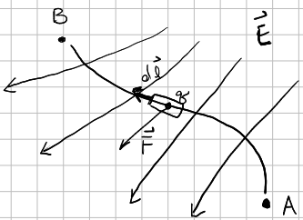
The force acting on the charge is \(\v{F} = q \v{E}\) at any point. Then, the work done on the charge agaisnt the action of the field is (hence, the negative sign),
\[W = - \int_{A}^{B} \v{F} \cdot d\v{l} = - q \int_{A}^{B} \v{E} \cdot d\v{l}\]In terms of the scalar potential,
\[W = q \int_{A}^{B} \del\Phi \cdot d\v{l} = q \int_{A}^{B} d \Phi = q (\Phi_{B} - \Phi_{A})\]where \(q\Phi\) can be interpreted as the potential energy of the test charge in an electrostatic field.
Note that the work done is path independent between the two points. Moreover, the potential is also the negative difference between the two points.
\[\int_{A}^{B} \v{E} \cdot d\v{l} = -( \Phi_{B} - \Phi_{A})\]If the path is closed, in other words, if the charge ends up back in the same place as point \(A\), then,
\[\oint \v{E} \cdot d\v{l} = 0\]We can apply Stoke’s theorem to obtain the \(\del \times \v{E} = 0\) result again.
\[\oint_{C} \v{A} \cdot d\v{l} = \int_{S} (\del \times \v{A}) \cdot \v{n} da\]Stoke’s Theorem: If \(\v{A} (\v{x})\) is a well-behaved vector field, \(S\) is and arbitrary open surface, and \(C\) is closed bounding \(S\), then the following holds,
where \(d\v{l}\) is a line element of \(C\), \(\v{n}\) is normal to \(S\), and \(C\) is the traversed path in a right-hand screw relative to \(\v{n}\).
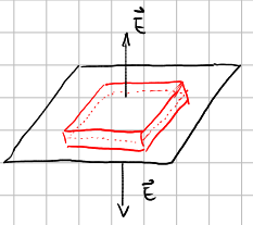
Consider a surface \(S\), with a unit vector \(\v{n}\) normal to the surface from side \(1\) to side \(2\). Using Gauss’s law, the electric field is written as the difference of the field of side \(1\) and the field of side \(2\). To elaborate, on one side of the surface, the electric field \(\v{E}_{1}\) normal to the surface is,
\[\oint_{S} \v{E}_{1} \cdot dS = \v{E}_{1} \oint_{S} dS = \v{E}_{1} A\]The charge enclosed in the gaussian surfrace takes the form of a surface charge density \(\sigma = \f{Q}{A}\), so the volume integral reduces down to a surface integral.
\[\f{1}{\eo} \int_{V} \sigma d^{3} a = \f{\sigma A}{\eo}\]However, the contribution of the electric field on the other side of the surface needs to be accounted for. As a result, a factor of \(2\) is added. The \(\v{E}\) flux through a surface is,
\[\v{E}_{1} 2A\]All together, Gauss’s law for a single surface charge distribution is,
\[\v{E}_{1} 2 A = \f{\sigma A}{\eo}\] \[\v{E}_{1} = \f{\sigma}{2\eo}\]In the presence of another charged surface (parallel plate configuration) of field \(\v{E}_{2}\), with an equal and opposite charge, the fields are a superposition,
\[\v{E}_{2} - \v{E}_{1} = \f{\sigma_{2}}{2\eo} - \f{-\sigma_{1}}{2\eo} = \f{\sigma}{\eo}\]The surface integral evalutes to \(A\) since the field lines through the Gaussian surface (a pillbox) are the only lines that contribute to the \(\v{E}\) flux through surface area \(A\).
Consider a single surface of charge density, \(\sigma(x)\) with a normal vector \(\v{n}\) through side \(1\) and side \(2\) of the surface. The electric field is given by,
\[(\v{E}_{2} - \v{E}_{1}) \cdot \v{n} = \f{\sigma}{\eo}\]where \(\sigma (x)\) is the surface charge density, measured in Coulombs per square meter. This tells us that there is a discontinuity of \(\sigma / \eo\) in the normal component of the electric field in the direction of \(\v{n}\).
The tangential components of the electric field follows that \(\oint \v{E} \cdot d\v{s} = 0\) since a rectangular path is taken with negligible ends and one side on either side of the boundary.
The scalar potential can be expressed in terms of the surface charge density and its infinitesimal element \(da\),
\[\Phi(\v{x}) = \f{1}{4\pi\eo} \int_{S} \f{\sigma(\v{x'})}{\abs \v{x} - \v{x'} \abs } da'\]The potential for volume or surface charge distributions are continuous everywhere since they are bounded by \(\v{E}\). However, in the case of point, line, or dipole layer charge configurations, continuous potentials are no longer the case.
Consider a dipole layer distribution on a surface \(S\). The figure below shows a surface \(S\) with a surface charge density \(\sigma(\v{x})\) and another surface \(S'\) with a surface charge equal and opposite, \(-\sigma(\v{x})\). We are interested in studying the potential due to the surfaces.
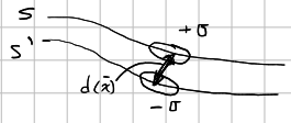
First, it is important to set up the limiting process for two surfaces as they close the distance between them. The dipole layer distribution of strength, \(D(\v{x})\) can be written in terms of a limit,
\[\lim_{d(\v{x}) \rightarrow 0 } \sigma(\v{x}) d(x) = D(\v{x})\]where the seperation, \(d(\v{x})\), between \(S\) and \(S'\) approaches \(0\), which allows the product to appoarch the limit \(D(\v{x})\).
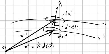
The potential due to two close surfaces is written in terms of its evaluation at origin \(O\).
\[\Phi(\v{x}) = \f{1}{4 \pi \eo} \int_{S} \f{ \sigma(\v{x'}) }{ \abs \v{x} - \v{x'} \abs } da' - \f{1}{4 \pi \eo} \int_{S'} \f{\sigma(\v{x'})}{\abs \v{x} - \v{x'} + \v{n} d \abs} da''\]Using the Taylor series expansion, the seperation term of the \(S'\), \(\abs \v{x} - \v{x'} + \v{n} d \abs^{-1}\) can be rewritten for an expression that takes the form \(\abs \v{x} + \v{a} \abs^{-1}\) where \(\abs \v{a} \abs \ll \abs \v{x} \abs\).
\[\f{1}{\abs \v{x} + \v{a} \abs } \equiv -\frac{1}{ \sqrt{x^{2} + a^{2} + 2\v{a} \cdot \v{x}} }\] \[= \f{1}{x} \bigg( 1 - \f{\v{a} \cdot \v{x}}{x^{2}} + ...\bigg)\] \[\f{1}{\abs \v{x} + \v{a} \abs } = \f{1}{x} + \v{a} \cdot \del (\f{1}{x}) + ...\]Expanding around \(d \rightarrow 0\) and applying \(D(x)\), the potential becomes
\[\Phi(\v{x}) = \f{1}{4 \pi \eo} \int_{S} D(\v{x'}) \v{n} \cdot \del' \bigg( \f{1}{ \abs \v{x} - \v{x'} \abs} \bigg) da'\]From here, we can define the dipole moment \(\v{p} = \v{n} D da'\). We aim to find the potential in the region just above the plane. In other words, the potential at \(\v{x}\) caused by dipole \(\v{p}\) at \(\v{x'}\) is,
\[\Phi(\v{x}) = \f{1}{4 \pi \eo } \f{ \v{p} \cdot ( \v{x} - \v{x'} ) }{ \abs \v{x} - \v{x'} \abs^{3} }\]Since many electrostatic problems involve finite regions of space with or without charge inside, boundary-value problems will eventually more rigorous treatment beyond simple cases (where one would apply the method of images). For more complex potentials, we can apply identities and theorems from Green’s Theorem to handle their boundary conditions. Recall the divergence theorem,
\[\int_{V} \del \cdot \v{A} d^{3}x = \oint_{S} \v{A} \cdot \v{n} da\]Let \(\v{A} = \phi \del \psi\). \(\v{A}\) is a well behaved vector field defined in the volume \(V\) and bounded by a closed surface \(S\). \(\phi\) and \(\psi\) are arbitrary scalar fields. Using the following divergence identity:
\[\del \cdot (\phi \del \psi) = \psi \del^{2} \psi + \del \phi \cdot \del \psi\]Dotting the divergence of a function into a unit vector is just the partial derivative taken with respect to the normal at the surface \(S\), directed outward from inside the volume \(V\).
\[\phi \del \psi \cdot \v{n} = \phi \f{\pd \psi}{ \pd n}\]By substitution, the identities from above results in Green’s first identity.
Green’s 1st Identity:
\[\int_{V} (\phi \del^{2} \psi + \del \phi \cdot \del \psi ) d^{3}x = \oint_{S} \phi \f{\pd \psi}{ \pd n} da\]
Green’s 2nd Identity:
\[\int_{V} (\phi \del^{2} \psi - \psi \del^{2} \phi) d^{3}x = \oint_{S} \bigg[ \phi \f{\pd \psi}{\pd n} - \psi \f{\pd \phi}{\pd n} \bigg] da\]
Two sets of equations need to kept in mind when solving electrostatic problems. That is, Laplace’s equation,
\[\del^{2} \phi = \del \cdot (\del \phi) = 0\]which states that the divergence of a scalar g
This also encompasses a class of functions, a twice continuously differentiable real-valued function is a harmonic function.
The importance of this equation comes from the fact that \(\del \times \v{E} = 0\) and that \(\v{E}\) can be written as the gradient of a scalar field \(-\del \phi\). Put simply, all three components of the electric field everywhere can be obtained without having to seperately evaluate three component partial differential equations!
Consider an grounded (\(\Phi = 0\)) infinite conducting plan. We aim to calculate the potential for the region just above the plane, where a charge is place at \((d, 0 ,0)\). We know that the total potential will be related to the charge placed at the region. However, the nothing is known about the charge induced for the surface. Hence, we apply the method of images as a way to fill out the rest of the picture for the charge configuration. The figure below shows the equivalent image, an equal and opposite “image” charge placed on the other side of the plane
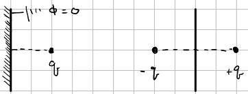
In essence, the solution should satisfy Poisson’s equation, \(\del^{2}\Phi = -\f{\rho}{\eo}\). This also involves the uniqueness theorem for Poisson’s equations, which states that for a large class of boundary condition, the gradient of every solution is the same. In other words, there is a unique electric field that can be obtained from a potential function such that the following boundary conditions are satisfied:
By placing the image charge at some distance \(a\), the potential can be readily solved for a two charge configuration.
\[\Phi(\v{x}) = \f{1}{4\pi\eo} \bigg[ \f{q}{\abs \v{x} - \v{x'_{1}} \abs} + \f{q'}{\abs \v{x} -\v{x'_{2}}\abs}\bigg]\] \[= \f{1}{4\pi\eo} \bigg[ \f{q}{\sqrt{ d^{2} + y^{2} + z^{2}}} + \f{q'}{ \sqrt{a^{2} + y^{2} + z^{2}} }\bigg] = 0\]The Dirichlet boundary condition requires that the potential vanishes at a, \(\Phi(\v{x} = a) = 0\), which is satified if the following is true:
These definitions are equal in magnitude and opposite. Thus, replacing a few variables from the statements above yields,
\[\Phi(\v{x}) = \f{1}{4\pi\eo} \bigg[ \f{q}{\sqrt{ (x-d)^{2} + y^{2} + z^{2}}} - \f{q'}{ \sqrt{ (x+d)^{2} + y^{2} + z^{2}} }\bigg]\]Not with a well-defined potential, the \(\v{E}\) field can be determined using \(\v{E}=-\f{\pd \Phi}{\pd x}\)
\[\v{E} = \f{q}{4\pi \eo} \bigg[ \f{(x-d)}{[(x - d)^{2} + y^{2} + z^{2}]^{3/2}} - \f{(x+d)}{[(-x+d)^{2} + y^{2} + z^{2}]^{3/2} } \bigg]\]Which can be used to evaluate the electric field at various distances, \(x\), from the conducting plane,
\[\v{E} \abs_{x=0} = -\frac{q}{4\pi \eo} \frac{2d}{[d^{2} + y^{2} + z^{2}]^{3/2}}\]The surface charge distribution can also be found using the following relationship:
\[\sigma = -\eo \f{\pd \Phi}{\pd x} = \eo \v{E}_{x} \abs_{x=0}\]where the partial derivative is taken with resepect to the normal component of the field.
Consider a conducting metal sphere of radius \(a\). The sphere is grounded. In other words, the potential of the sphere is held at the same potential as the point at \(\infty\) and arbitrary charges of either sign can flow onto the object from infinity to maintain ground. We aim to derive an expression for the potential \(\Phi(\v{x})\) such that \(\Phi(\abs x \abs = a) = 0\) by applying the method of images.
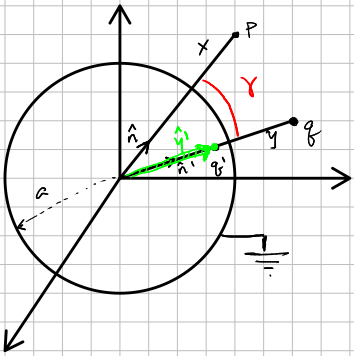
Evaluating the potential at point \(P\), the symmetry of the sphere requires that the image charge ,\(q'\), is to be placed in line with the vector pointing from the origin to \(q\). So the potential due to the charges is,
\[\Phi(\v{x}) = \f{1}{4\pi\eo}\bigg[ \f{q}{ \abs \v{x} - \v{y} \abs} + \f{q'}{\abs \v{x} - \v{y'} \abs} \bigg]\]Rewriting the seperation vectors in terms of their unit vector components: \(\h{n}\) points in the direction \(\v{x}\) and \(\h{n}'\) points in the direction of \(\v{y}\).
\[\Phi(\v{x}) = \f{1}{4\pi\eo} \bigg[ \f{q}{ \abs x\h{n} - y\h{n'} \abs} + \f{q'}{\abs x\h{n} - y' \h{n'} \abs} \bigg]\]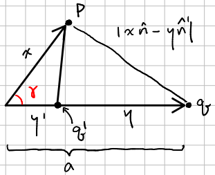
Again, the choice of \(q'\) and \(\abs \v{y'} \abs\) will be dependent on the fact that \(\Phi(\abs \v{x} \abs = a) = 0\), the goal in mind is making both charge (and their seperation terms) equal and opposite such that Poisson’s equations are satisfied.
Reworking the equation may provide a better view of what variables need to be involved to satisfy the boundary conditions. At \(\v{x}=a\) for \(\Phi(a)\). Pulling out the first terms in the first term and the second,
\[\Phi(x=a) = \f{1}{4\pi\eo} \bigg [\f{q}{a \abs \h{n} - \f{y}{a} \h{n'} \abs } + \f{q'}{y' \abs \h{n'} - \f{a}{y'} \h{n} \abs} \bigg] = 0\]Again, the statement is only true if quantities are:
\[\f{q}{a} = -\f{q'}{y'}\] \[\f{y}{a} = \f{a}{y'}\]The relationship between the position and magntitude of the charges then follow,
\[q' = - \f{a}{y} q\] \[y' = \f{a^{2}}{y}\]The seperation vector can be rewritten as follows,
\[\abs \h{n} - \h{n}' \abs =\] \[= \sqrt{ (\h{n} - \h{n}' )^{2} }\] \[= \sqrt{ \h{n} \cdot \h{n} + \h{n} \cdot \h{n}' - 2 \h{n} \cdot \h{n} }\] \[= \sqrt{1 + 1 - 2 \cos{\gamma}}\]We can obtain two relationships regarding the seperation vectors:
\[\abs \h{n} - \f{y}{a} \h{n}' \abs = \sqrt{1 + \f{y^2}{a^2} - 2\f{y}{a} \cos{\gamma} }\] \[\abs \f{a}{y} \h{n} - \h{n}' \abs = \sqrt{ \f{a^{2}}{y'^{2}} + 1 + 2\f{a}{y'}\cos{\gamma}}\]This may be easier to see if we evaluate the equation at \(x=a\),
\[\Phi(x=a) = \f{1}{4\pi\eo} \bigg[ \f{q}{ a \abs \h{n} - \f{y}{a} \h{n}' \abs } + \f{q'}{ y' \abs \f{a}{y'} \h{n} - \h{n}' \abs } \bigg]\] \[\Phi(x=a) = \f{1}{4\pi\eo} \bigg[ \f{1}{ \sqrt{x^{2} + y^{2} - 2xy \cos{\gamma} } } + \f{a/y}{ \sqrt{ x^{2} + (\f{a^{2}}{y})^{2} + 2x\f{a^{2}}{y}\cos{\gamma}} } \bigg]\]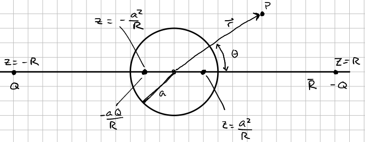
Consider a conducting sphere of radius \(a\) in a uniform electric field \(E_{0}\) provided by placing . two charges \(\pm Q\) at infinity, located at \(z = \mp R\).
Before writing down the potential due to the configuration, it may be helpul to examine the separation vectors and apply a Taylor expansion for \(r \ll R\).
\[\abs \v{r} - \v{R} \abs^{-1} = \f{1}{\sqrt{r^{2} + R^{2} - 2rR\cos{\theta}}}\] \[= \f{1}{R \sqrt{1 + r^{2}/R^{2} - \f{2r}{R}\cos{\theta}}}\]Again, based on the conditions of the expansion \(\f{r}{R} \ll 1\),
\[\approx \f{1}{R} \bigg(1 + \f{r}{R}\cos(\theta) \bigg)\]Using Green’s theorem, the generalized solution for a finite volume \(V\) with Dirichlet or Neumann boundary conditions bounded by a surface \(S\) can be written as,
\[\Phi(\v{x}) = \f{1}{4\pi\eo} \int_{V} \rho(\v{x}') G(\v{x}, \v{x}') d^{3}x' + \f{1}{4\pi} \oint_{S} \bigg[ G(\v{x},\v{x}') \f{\pd \Phi}{\pd n'} - \Phi(\v{x}') \f{\pd G(\v{x}, \v{x}')}{\pd n'} \bigg] da'\]For a function that takes the form of \(\f{1}{\abs \v{x} - \v{x}' \abs}\),
\[\del'^{2} G(\v{x},\v{x}') = -4\pi\delta(\v{x} - \v{x}')\]where
\[G(\v{x},\v{x}') = \f{1}{\abs \v{x} - \v{x}' \abs} + F(\v{x},\v{x}')\]We can readily apply this to a spherical configurations using the method of images. We can define point \(P\) with vector \(\v{x}\) as the point at which the potential is being evaluated, and \(P'\) with vector \(\v{x}'\) as the unit source. Not drawn in the figure is an arbritary image charge with a \(\v{x}''\) component to help with image-boundary conditions. Writing the appropriate Green function,
\[G(\v{x}, \v{x}') = \f{1}{\abs \v{x} - \v{x}' \abs} + \f{c}{\abs \v{x} - \v{x}'' \abs }\]where \(c\) is an arbitrary constant that is representative of an image charge such that we can apply a Dirichlet boundary conditions (\(G(\v{x}, \v{x}') = 0\) on the surface) to obtain the following Green function:
\[G(\v{x}, \v{x}')= \f{1}{\abs \v{x} - \v{x}' \abs} - \f{a}{ x' \abs \v{x} - \f{a^{2}}{x'^{2}} \v{x}' \abs}\]with \(c = \f{a}{x}\) and \(\abs \v{x}'' \abs = \f{a^{2}}{x'}\), whose form should look like the potential in an image problem. Expanding the vectors into their scalars,
\[G(\v{x}, \v{x}') = \f{1}{( x^{2} + x'^{2} - 2xx'\cos\gamma )^{1/2}} - \f{1}{( \f{x^{2} x'^{2}}{a^{2}} + a^{2} - 2xx'\cos\gamma )^{1/2}}\]The Laplace equation in rectangular coordinates is written as:
\[\del^{2} \Phi = \f{\pd^{2} \Phi}{\pd x^{2}} + \f{\pd^{2} \Phi}{\pd y^{2}} + \f{\pd^{2} \Phi}{\pd z^{2}} = 0\]The general solution to the partial differential equation can be found in terms of ordinary differential equations, where the solution is written as a product of three functions.
\[\Phi(x,y,z) = X(x) Y(y) Z(z)\]substituting \(\Phi\) into the Laplace equation and dividing through by \(XYZ\),
\[\f{1}{X} \f{d^{2} X}{d x^{2}} + \f{1}{Y} \f{d^{2} Y}{d y^{2}} + \f{1}{Z} \f{d^{2} Z}{d z^{2}} = 0\]Now that the equation is in terms of total derivatives since each function involves its respective variable, the next thing to do is to each term a constant since each term holds arbitrary values for each independent coordinate.
\[\f{1}{X} \f{d^{2} X}{d x^{2}} + \alpha^{2} = 0\] \[\f{1}{Y} \f{d^{2} Y}{d y^{2}} + \beta^{2} = 0\] \[\f{1}{Z} \f{d^{2} Z}{d z^{2}} - \gamma^{2} = 0\]Where \(\gamma^{2} = \alpha^{2} + \beta^{2}\) Since we know what to expect for the solutions of the differential equations, the choice of positive \(\alpha\) and \(\beta\) values provide a large class of solutions to the Laplace equation.
\[\Phi = e^{\pm i \alpha x} e^{\pm i \beta y} e^{\pm \sqrt{\alpha^{2} + \beta^{2} } }\]The Laplacian in terms of radial coordinates is written as:
\[\f{1}{r^{2}} \f{\pd}{\pd r} \bigg( r^{2} \f{\pd \Phi}{\pd r} \bigg) + \f{1}{r^{2} \sin\theta} \f{\pd }{\pd \theta} \bigg( \sin\theta \f{\pd \Phi}{\pd \theta} \bigg) + \f{1}{r^{2} \sin^{2}\theta} \f{\pd^{2} \Phi}{\pd \phi^{2}} = 0\]where the potential is assumed to be of the form:
\[\Phi = \frac{U(r)}{r} P(\theta) Q(\phi)\]Consider an electric dipole that consists of two equal and opposite charges seperated by some distance, \(\pm q\) and \(d\) respectively.
The dipole vector is defined as,
\[\v{p} = q \v{d}\]The two seperation vectors for the charges can be expanded into their scalar forms,
\[\v{r}_{+} = \v{r} - \f{d}{2} = (r^{2} + \f{d^{2}}{4} - \v{r} \cdot \v{d})^{1/2}\] \[\v{r}_{-} = \v{r} + \f{d}{2} = (r^{2} + \f{d^{2}}{4} + \v{r} \cdot \v{d})^{1/2}\]where \(\v{r} \cdot \v{d} = r d \cos(\gamma)\).
The potential in terms of multipole moments, \(q_{lm}\), and spherical harmonics, \(Y_{lm} (\theta, \phi)\), is
\[\Phi(r, \theta, \phi) = \f{1}{4\pi\eo} \sum_{l=0}^{\infty} \sum_{m=-l}^{+l} \f{4\pi}{2l+1} \f{Y(\theta,\phi)}{r^{l+1}}\]We can map these this multipole potential to the Coulomb potential,
\[\Phi(\v{r}) = \f{1}{4\pi\eo} \int \f{\rho(\v{r'})}{\abs \v{r} - \v{r'} \abs} d^{3}\v{r'}\]where the seperation term can be expanded in terms of its spherical harmonics (which are a complete orthonormal set),
\[\f{1}{\abs \v{r} - \v{r'} \abs} = 4\pi \sum_{l=0}^{\infty} \sum_{l=-m}^{+m} \f{1}{2l+1} \f{r^{l}_{>}}{r^{l+1}_{<}} Y^{*}(\theta', \phi') Y(\theta,\phi)\]plugging the \(1/ \abs \v{r} - \v{r'} \abs\) expansion into the potential derived from Gauss’ law,
\[\f{1}{\eo} \sum_{l,m} \f{1}{2l+1} \bigg[ \int Y^{*}_{lm} (\theta', \phi') r^{'l} \rho (\v{r'}) d^{3} \v{r'} \bigg] \f{Y_{lm}(\theta, \phi)}{r^{l+1}}\]where the multipole moments are contained in the term,
\[q_{lm} = \int Y^{*}_{lm} (\theta', \phi') r^{'l} \rho (\v{r'}) d^{3} \v{r'}\]which can be evaluated from a given charge distribution \(\rho(\v{r'})\). For example, the monopole moment, for \(l=0\),
\[q_{00} = \f{1}{\sqrt{4\pi}} \int \rho(\v{r'}) d^{3} \v{r'} = \f{q}{\sqrt{4\pi}}\]The dipole moment is the next term in the expansion, where \(l=1\). Note that there are indicies \(m\) that will provide the three component \(x,y,z\) terms of the dipole,
\[q_{11} = - \sqrt{\f{3}{8\pi}} \int (x' - 'y') \rho(\v{r'}) d^{3}\v{r'} = -\sqrt{\f{3}{8\pi}} (P_{x} - 'P{y})\] \[q_{10} = \sqrt{\f{3}{4\pi}} \int z' \rho(\v{r'}) d^{3} r' = \sqrt{\f{3}{4\pi}} P_{z}\]where the physical interpretation of the dipole moment is,
\[\v{P} = \int \v{r'} \rho(\v{r'}) d^{3} \v{r'}\]Usually, these multipole moments can be further expanded, but generally, it is enough to stop at \(l=2\), the quadrupole terms.
Many of the magnetostatics naturally take the form of electrostatics equations, for instance both the divergence and curl can be written as:
\[\del \cdot \v{B} = 0\]If a moving charge density, \v{J}, is present,
\[\del \times \v{B} = \mu \v{J}\]where the current, \(I\) is,
\[I = \int \v{J} \cdot \h{n} da\]We can convert these into integral form and arrive at Ampere’s law, where \(\del \times \v{B}\) becomes,
\[\oint \v{B} \cdot dl = \mu_{0} \int_{S} \v{J} \cdot da = \mu_{0} I_{enc}\]This looks similar to gauss’s law for an enclosed charge \(Q_{enc}\)
Consider a long straight wire carry a current \(I\). Much like a Gaussian surface, we draw an Amperian loop around the wire such that we exploit the symmetry of the wire. This allows us to move \(\v{B}\) out of the integral since it is a constant.
\[\oint_{C} \v{B} \times dl = B \int dl = B (2\pi r) = \mu_{0} I\] \[\v{B} = \f{mu_{0} I }{2 \pi r} \h{\phi}\]Recall the potentials in electro statics. The curl, \(\del \times \v{E}=0\) is related to a scalar potential \(\v{E} = -\del\Phi\).
However, for magnetostatics, the potential takes the form of a vector potential, where the divergence is,
\[\del \cdot \v{B} = 0\]with
\[\v{B} = \del \times \v{A}\]Consider a current going through a loop with an induced magnetic field \(\v{B}\)
\[d\v{B} = k I \f{d\v{l} \times \v{x} }{ \abs \v{x} \abs^{3}}\] \[\v{B} = k \int I \f{(d\v{l} \times \v{x})}{\abs \v{x} \abs^{3}}\]where \(k = \f{\mu_{0}}{4\pi} = 10^{-7} \f{N}{A^{2}}\)
For a long straight wire,
\[d\v{l} \times \v{x} = dl x \sin\theta\] \[= dlx(\f{R}{x}) = dl R\] \[\v{B} = \f{\mu_{0} I R}{4\pi} \int_{-\infty}^{\infty} \f{dl}{(R^{2} + l^{2})^{3/2}} = 2/R^{2}\] \[\v{B} = \f{\mu_{0} I}{2\pi R^{2}}\]There are three ways to integrate for the force,
Using a standard differential line integral,
\[\v{F} = \int I (d\v{l} \times \v{B})\]Using surface current, \(\v{K}\), in units of \(A/m\),
\[\v{F} = \int da (\v{K} \times \v{B})\]and using current density, \(\v{J}\), in units of \(A/m^{2}\)
For two long parallel wires, we can calculate a force per unit length,
\[\f{d\v{F}}{dl} = \f{\mu_{0}}{2\pi} \f{I_{1} I_{2}}{d}\]The equation above should look familiar. It’s essentially Coulomb’s law put in terms of current.
The scalar potentials and associated fields for \(\v{B}\) and \(\v{E}\) are the same integrals over the seperation vector, \(1/(\v{x} - \v{x'})\). The difference between the two is the “density” that the integral is calculated over. To elaborate, \(\v{B}\) integrals will be a function of the current density \(\v{J}\) whereas \(\v{E}\) will be an integral over the the charge density \(\rho\).
The vector potential, \(\v{A}\), is evaluated as
\[\v{A}(\v{x}) = \f{\mu_{0}}{4\pi} \int \f{\v{J}(\v{x})}{\abs \v{x} - \v{x'} \abs^{3}}d^{3}\v{x'}\]and the magnetic field, \(\v{B}\),
\[\v{B}(\v{x}) = \f{\mu_{0}}{4\pi} \int \v{J}(\v{x}) \times \f{(\v{x} - \v{x'})} {\abs \v{x} - \v{x'} \abs^{3}}d^{3}\v{x'}\]Due to gauge invariance, the gradient to a scalar can be added to \(A\) without changing \(B\). Let \(\v{A'} = \v{A} + \del \Omega\), where \(\v{A'}\) is a modified vector potential,
\[\v{B'} = \del \times \v{A'} = \del \times \v{A} + \del \times \del \Omega = \del \times \v{A} = \v{B}\]The reason why this works is because taking the curl of the gradient of the potential yields, \(\del \times \del \Omega = 0\).
(Helmholtz Theorem) In order to fully define any vector field, the curl, \(\del \times \v{A}\), and the divergence, \(\del \cdot \v{A}\), need to be fully specified.
For instance, the Coulomb gauge specifies that \(\del \cdot \v{A} = 0\)
Consider a conductive cylinder with some cross-sectional area \(A\). Let \(dx\) be an infinitesimal section of the cylinder. The number of electrons passing through the cylinder is: \(n_{e^{-}} = - e N A dx\)
Taking the time-derivative yields the current:
\[I = \frac{d Q}{dt} = - e N A \frac{dx}{dt}\]Dividing through by \(A\) gives current density, \(J\):
\[\frac{I}{A} = J = - e N v\]Using out definition of \(J\) from above, we put the equation of motion of an electron in a metal in terms of velocity, \(\vec{v}\) and plug in \(\vec{v}\) in terms of \(J\).
\[m \frac{d^{2}\vec{r}}{dt^{2}} = - e \vec{E} - \gamma m \frac{d\vec{r}}{dt}\]Consider a simple dielectric, a non-conducting (no free-charges) material whose properties are isotropic. The application of an \(\vec{E}\) field produces an induced dipole, a slight shift in the electron cloud relative to the nucleus.
The dipole moment can be defined as:
\[\vec{p} = - q \vec{r}\]where \(q\) is the magnitude of the displace charge and \(\vec{r}\) points from the effective negative charge center relative to the effective positive charge center in a dipole.The direction of the dipole moment points from the negative to positive charges.
The Polarization of the medium is defined as the collective dipole moment per unit volume:
\[\vec{P} = - N e \vec{r}\]where \(N = n/V\), the number of elementary dipoles per unit volume and \(e\) is the magnitude electron charge.
We can start out with a simple Hooke’s law model where electrons are bound by spring-like forces to a fixed nucleus. Like a spring, the forces binding the electrons to the nucleus has a restoring force that is proportional to the displacement and is oppositely directed.
\[F_{s} = -K_{s} \vec{r}\]Adding another layer to the model, due to the intertions of neighboring atoms and thermal energy loss in the presence of an alternating \(E\) field, an oscillating electron can be modelled after a damped harmonic oscillator with a “frictional” force proportional to velocity.
Thus, the resulting equation of motion for this model is:
\[-K_{s} \vec{r} - m \gamma \frac{d \vec{r}}{dt} - e \vec{E} = m \frac{d^{2} \vec{r}}{dt^{2}}\]where \(K_{s}\) is the force constant of an effective spring, \(m\) is the electron mass and \(\gamma\) is the frictional constant with dimensions \(s^{-1}\).
A small detour: Negligible \(F_{\vec{B}}\)
Notice that the equation of motion for our electron-nucleus model does not include the force provided by a \(\vec{B}\) field. Let’s find the ratio of the forces of the \(\vec{E}\) and \(\vec{B}\) fields.
\[\frac{F_\vec{E}}{F_\vec{B}} = \frac{e |E|}{v |B|}\]Recall that the speed of light is a ratio of the \(\vec{E}\) and \(\vec{B}\) fields i.e. \(c = \frac{E}{B}\). Using that definition:
\[\frac{F_\vec{E}}{F_\vec{B}} = \frac{c}{v}\]Here \(c = 3 \times 10^{8} m/s \gg v\). Hence, \(F_{\vec{B}}\) is negligible.
A small detour II: static \(\vec{E}\) fields
In the special case of an applied \(\vec{E}\) field that is static, the dipoles do not oscillate, both \(\frac{d^{2} \vec{r}}{dt^{2}}\) and \(\frac{d \vec{r}}{dt}\) are both \(0\).
Using this result, static polarization is defined as:
\[\vec{P} = \frac{N e^{2} \vec{E}}{K_{s}}\]Suppose that \(\vec{E}\) is a harmonic field given by:
\[\vec{E} = \vec{E}_{0} e^{-i \omega t}\] \[\vec{r} = \vec{r}_{0} e^{-i \omega t}\]The derivatives for the differential equation:
\[\frac{d\vec{r}}{dt} = - i \omega r_{0} e^{-i \omega t} = - i \omega \vec{r}\] \[\frac{d^{2} \vec{r}}{dt^{2}} = - \omega^{2} r_{0} e^{- i \omega t} = - \omega^{2} \vec{r}\]Solving…
\[- K_{s} \vec{r} - m \gamma (- i \omega \vec{r} ) - e \vec{E} = m ( - \omega^{2} \vec{r} )\] \[\vec{r} = \frac{e \vec{E}}{- m \omega^{2} - i m \omega \gamma + K_{s}}\]Substituting this into the Polarization equation yields:
\[\vec{P} = \bigg( \frac{Ne^{2}}{-m \omega^{2} - i m \omega \gamma + K_{s}} \bigg) \vec{E}\]The index of refraction can be represented as the ratio between the speed of light in vacuum versus in a medium:
\[n = \frac{c}{v}\]Recall the speed of light (in vacuum) can be written as:
\[c = \frac{1}{\sqrt{\mu_{0} \epsilon_{0}}}\]whereas in a medium:
\[v = \frac{1}{\sqrt{\mu_{0} \epsilon }}\]Combining the two definitions above:
\[n = \frac{\sqrt{\mu_{0} \epsilon}}{\sqrt{\mu_{0} \epsilon_{0}}}\] \[n = \sqrt{\frac{\epsilon}{\epsilon_{0}}} = \sqrt{\epsilon_{r}}\]Where \(\epsilon_{r}\) is the relative permittivity.
A mathematically improper function, the delta function in one dimension is,
\[\delta (x - a)\]with the property,
\(\delta (x-a) = 0\) for \(x \neq a\)
\(\int \delta (x - a) dx = 1\) for regions \(x = a\) and \(0\) otherwise
Some other properties of the delta function are shown below…
\[\int f(x) \delta(x - a) dx = f(a)\] \[\int f(x) \delta' (x-a) dx = \int [ f(x) \delta(x) ]' dx - \int f'(x) \delta(x) dx = \f{d}{dx} [f(x) \delta(x) dx] - f'(0) ]= - f'(a)\] \[\delta(kx) = \f{1}{ \abs k \abs} \delta(x)\]Proof:: Let y=kx, \(\int_{-\infty}^{+\infty} f(x) \delta(kx) dx = \pm \int_{-\infty}^{+\infty} f(y/k) \delta(y) \f{dy}{k}\)
\[= \pm \f{1}{k} \int_{-\infty}^{+\infty} f(y/k) \delta(y) dy = \pm \f{1}{|k|} f(0) = \int_{-\infty}^{+\infty} f(x) \f{\delta(x)}{|k|} dx\]
likewise,
\[\delta(ax-b) = \delta(a (x - \f{b}{a})) = \f{1}{|a|} \delta(x-\f{b}{a})\]
Charge distribution:
\[\del^{2} \Phi = -\f{\rho}{\eo}\]Conducting Boundary conditions:
\[\del^{2} \Phi = 0\]Classical Electrodynamics, J.D. Jackson
Introduction to Electrodynamics, D.J. Griffith