Important Theorems and Equations for Classical Mechanics
\(\let\vec\mathbf\) \(\newcommand{\v}{\vec}\) \(\newcommand{\d}{\dot{}}\) \(\newcommand{\abs}{\rvert}\) \(\newcommand{\h}{\hat}\) \(\newcommand{\f}{\frac}\) \(\newcommand{\~}{\widetilde}\) \(\newcommand{\<}{\langle}\) \(\newcommand{\>}{\rangle}\)
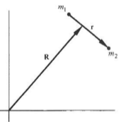
Consider a monogenic system such as the one below:
The Lagrangian will have the form:
\[L = T ( \dot{\vec{R}}, \dot{\vec{r}} ) - U (\vec{r},\dot{\vec{r}},... )\]We choose the two generalized coordinates, \(q_{i}\):
\[\vec{R}_{CM} = \frac{m_{1} \vec{r}_{1} + m_{2} \vec{r}_{2}}{m_{1}+m_{2}}\] \[\vec{r} = \vec{r}_{2} - \vec{r}_{1}\]\(R_{CM}\) points to the center of mass of the system and \(\vec{r}\) is the distance between \(m_{1}\) and \(m_{2}\).
It is also worth defining vectors relative to the center of mass:
\[\vec{r}_{1}' = \vec{r}_{1} - R_{CM}\] \[\vec{r}_{2}' = \vec{r}_{2} - R_{CM}\]Recall that the total kinetic energy, \(T\) can be decomposed into motion components of the center of mass,\(T_{CM}\), and motion relative to the center of mass, \(T_{rcm}\).
\[T = T_{CM} + T_{rcm}\]Center of mass kinetic energy is straightforward:
\[T_{CM} = \frac{1}{2} (m_{1} + m_{2}) \dot{\vec{R}}_{CM}^{2}\]Now, before dealing with \(T_{rcm}\), \(\vec{r}\) should be expressed in terms of \(\vec{r}_{1}'\) and \(\vec{r}_{2}'\). TO do this we take advantage of center of mass coordinates relative to the center of mass, which is just a zero vector:
\[m_{1} \vec{r}_{1}' + m_{2} \vec{r}_{2}' = \vec{0}\]Combining this with \(\vec{r} = \vec{r}_{2} - \vec{r}_{1}\), we obtain our coordinates relative to the center of mass in terms of \(\vec{r}\):
\[\vec{r}_{1}' = - \frac{m_{2} \vec{r}}{m_{1} + m_{2}}\] \[\vec{r}_{2}' = \frac{m_{1} \vec{r}}{ m_{1}+m_{2}}\]Now, setting up \(T_{rcm}\),
\[T_{rcm} = \bigg[ \frac{1}{2} m_{1} \bigg( \frac{m_{2}}{ m_{1} + m_{2} } \bigg)^{2} \bigg] \dot{\vec{r}}^{2} = \frac{1}{2} \bigg( \frac{m_{1} m_{2}}{ m_{1} + m_{2}} \bigg) \dot{\vec{r}}^{2}\]Let \(\mu = \frac{m_{1} m_{2}}{m_{1} + m_{2}}\), the reduced mass. The term “reduced” is given because it reduces motion about the center of mass of two objects down to one. T_{rcm} then simplifies to ,
\[T_{rcm} = \frac{1}{2} \mu \dot{\vec{r}}^{2}\]The Lagrangian with all its terms is:
\[L = \frac{m_{1} + m_{2}}{2} \dot{\vec{R_{CM}^{2}}}+ \frac{1}{2} \frac{m_{1} m_{2}}{m_{1} + m_{2}} \dot{\vec{r}}^{2} - U(\vec{r}, \dot{\vec{r}}, ...)\] \[L = \frac{m_{1} + m_{2}}{2} \dot{\vec{R_{CM}^{2}}}+ \frac{1}{2} \mu \dot{\vec{r}}^{2} - U(\vec{r}, \dot{\vec{r}}, ...)\]Notice that the Lagrangian is independent of \(R_{CM}\), which means \(\frac{\partial L}{\partial R_{CM}} = 0\). In other words, \(R_{CM}\) is cyclic/ignorable. Therefore simplifying the Lagrangian to:
\[L = \frac{1}{2} \mu \dot{\vec{r}}^{2} - U(\vec{r}, \dot{\vec{r}}, ...)\]This substantially simplifies the system, there are 3 degrees of freedom, described by \(\vec{r}\), and it turns out that this Lagrangian is the same for a point particle of mass \(\mu\) in a potential \(U(r)\)!
Let us work with the same reduced example: A particle of mass \(\mu\) orbiting a central potential.
Due to spherical symmetry, the angular momentum is given by:
\[L = \mu \vec{r} \times \vec{v} = constant\]\(L = constant\) and is conservered. \(\vec{r}\) and \(\vec{v}\) lie on the same plane, and are perpendicular to \(L\). This is to say that, it’s essentially a 2-D problem.
*note the change in notion, previous notes may have used \(U(r)\) as potential but now it’s \(V(r)\) .
The Lagrangian to this system is:
\[L(\vec{r}, \theta, \dot{\vec{r}}, \dot{\theta}) = \frac{\mu}{2} (\dot{\vec{r}^{2}} + \vec{r} \dot{\theta}^{2}) - V(\vec{r} )\]To simplify this Lagrangian a bit, we can make \(\mu = 1\). We can do this without loss of generality since all equations of motion will depend on \(\mu\).
We can say something about the momentum conjugate to \(\theta\), that is; the Lagrangian does not depend on \(\theta\), \((\frac{\partial L}{\partial \theta} = 0)\), and therefore \(\theta\) is cyclic and \(P_{\theta}\) is conserved.
\[P_{\theta} = \vec{r}^{2} \dot{\theta} = l = constant\]This is fantastic since one degree of freedom (\(\theta\)) has been eliminated. So with that, there are two observations to take note of.
where \(\frac{\partial L}{\partial \vec{r}} = r \dot{\theta} - \frac{dV}{d\vec{r}}\).
Notice that this is the same system of equation for a point mass in a central potential. Another example of the dynamics of a binary system reducing to a single point mass in a fixed potential!
Simplifying:
\[constant = H = \frac{\dot{r}^{2}}{2} + \frac{r^{2} \dot{\theta}}{2} + V(r)\]This energy equation is almost there. As it stands, the potential is dependent on the radius \(r\). However, \(\dot{\theta}\) still needs to be dealt with. We take advantage of an earlier definition, namely, the conserved momentum conjugate to \(\theta\), \(\vec{r}^{2} \dot{\theta} = l\) and substitute it into \(\dot{\theta}\).
\[H = \frac{1}{2} (\dot{r}^{2} + \frac{l^{2}}{r^{2}} ) + V(r)\]Remember that \(H\) is still constant, we can solve for \(\dot{r}\):
\[\bigg( \frac{dr}{dt} \bigg)^{2} = 2 ( E - V(r) ) \frac{l^{2}}{r^{2}}\]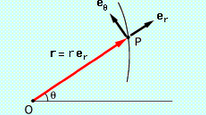
Let vector \(\vec{r}\) be the vector pointing from the origin to the particle.
\[\vec{r} = \hat{i} \vec{x} + \hat{j} \vec{y}\]Recall that \(x = r \cos(\theta)\) and \(y = r \sin(\theta)\)
\[\vec{r} = \hat{i} \cos(\theta) + \hat{j} \sin(\theta)\]Apply a small change \(d\vec{r}\), not a rate of change \(\frac{d\vec{r}}{dt}\)
\[d\vec{r} = \hat{i} (\cos\theta d\vec{r} - \vec{r} \sin\theta d\theta) + \hat{j} (\sin\theta d\vec{r} + \vec{r} \cos\theta d\theta )\]after distributing and collecting \(d\vec{r}\) and \(d\theta\) terms:
\[d\vec{r} = ( \hat{i} \cos\theta + \hat{j}\theta) d\vec{r} + (-\hat{i} \sin\theta + \hat{j} \cos\theta ) \vec{r} d\theta\]We can make use of some \(\hat{e}\) unit vector definitions where:
\(\hat{e}_{r} = \hat{i} cos\theta + \hat{j} \sin\theta\) is the radial term
\(\hat{e}_{\theta} = - \hat{i} \sin\theta + \hat{j} \cos\theta\) is the angular term
From here we obtain two polar equations for radial position and velocity:
\[d\vec{r} = \hat{e}_{r} d\vec{r} + \hat{e}_{\theta} \vec{r} d\theta\] \[\frac{d \vec{r}}{dt} = \hat{e}_{r} \frac{d\vec{r}}{dt} + \hat{e}_{\theta} \vec{r} \frac{d\theta}{dt} \rightarrow \vec{v} = \hat{e}_{r} \dot{r} + \hat{e}_{\theta} \vec{r} \dot{\theta}\]Recall that central forces (i.e. gravity, coloumbic forces) are forces that do not depend on direction, only position, \(V(r)\). Recently, we found that when tackling central force problems, one dimension is eliminated since angular momentum is conserved, or \(L = constant\).
Reconsider the Lagrangian (but this time, we just call the reduced mass \(\mu=m\) for generality:
\[L(\vec{r}, \theta, \dot{\vec{r}}, \dot{\theta}) = \frac{m}{2} (\dot{\vec{r}^{2}} + \vec{r} \dot{\theta}^{2}) - V(\vec{r} )\]Applying the Euler-Lagrange equation to the two generalized coordinates, \(r\) and \(\theta\), along with the equation derived from \(\theta\) being cyclic (also a first integral), gives us some equations of motion:
\[\frac{\partial L}{\partial r} - \frac{d}{dt} \bigg( \frac{\partial L}{\partial \dot{r}} \bigg) = 0\] \[\frac{\partial L}{\partial \theta} - \frac{d}{dt} \bigg( \frac{\partial L}{\partial \dot{\theta}} \bigg) = 0\]Recognizing that \(\frac{\partial L}{\partial \dot{\theta}}\) is some form of generalized momentum, we can take the time derivative, which gives us another equation of motion:
\[\dot{p}_{\theta} = \frac{d}{dt} \frac{\partial L}{\partial \dot{\theta}}= \frac{d}{dt} (m r^{2} \dot{\theta} ) = l\]where \(l\) is the constant magnitude of angular momentum. This is pretty important since it will be used throughout the section on central forces. The magnitude of the angular momentum is given by:
\[l = mr^{2} \dot{\theta}\][insert picture of angle sweep here]
Recall \(ds = r d\theta\).
\[r \dot{} ds = r ( r d\theta ) = r^{2} d\theta\]We find that this angle sweep is effectively calculating an area and divide by 2 (since the “sweep” begins as a square, and we cut it in half to form the triangle swept).
\[\f{dA}{dt} = \f{1}{2} r^{2} \f{d\theta}{dt} = \f{1}{2} r^{2} \dot{\theta}\]This draws out an “Area velocity” which is in the form of Kepler’s First Law.
As is standard in extracting equations of motion out of an Euler-Lagrange equation, we take two derivatives of \(L\) and plug back in. In this case, we obtain
\[m \ddot{r} - m r \dot{\theta} = f(r)\]we can replace \(\theta\) using out definition of the magnitude of angular momentum \(l = mr\dot{\theta}\):
\[m\ddot{r} - mr (\f{l}{mr^{2}} )= f(r)\]Which yields the radial equation to the central force problem:
\[m \ddot{r} - \f{l^{2}}{mr^{3}} = f(r)\]Simply flipping the sign in the Lagrangian gives us the energy of the system:
\[E = T + V = \f{1}{2} m (\dot{r}^{2} + r^{2} \dot{\theta}^{2} ) + V{r}\]just as we did for the radial equation, we use the definition of \(l\), and after some algebra, the energy equation looks something like:
\[E = \f{1}{2} m \dot{r}^{2} + \f{1}{2} \f{l}{mr^{2}} + V(r) = const\]This would be can solve for the “second integral”, by solving for \(\dot{r}\) in the energy equation:
\[\dot{r} = \big[ E - V(r) + \f{1}{2} \f{l^2}{mr^{2}} \big]^{1/2} \f{2}{m} = \f{dr}{dt}\]This integral can be evaluated using seperation of variables of course and we arrive at two master equations one for \(t(r)\) and another for \(\theta(t)\):
\[\int^{t}_{0} dt = \int^{r}_{r_{0}} \frac{dr}{ \f{2}{m} \big[ E - V(r) + \f{1}{2} \f{l^2}{mr^{2}} \big]^{1/2} }\] \[\theta (t) = \f{l}{m} \int^{t}_{0} \f{dt}{r^{2}} + \theta_{0}\]However, we cannot go any further for now since the potential energy \(V(r)\) has not been specified.
A statistical theorem in nature, the virial theorem is a general equation that relates the average kinetic energy of in a system of discrete particles.
For a system of particles, recall that the force is defined as:
\[\dot{\vec{p}}_{i} = \vec{F}_{i}\]We introduce a quantity, \(G\), since (I’m assuming) we want to form an equation about the kinetic energy of the system. Summing over the system of particles, \(G\), and taking the total time derivative:
\[G = \sum_{i} p_{i} \dot{} r_{i}\] \[\frac{dG}{dt} = \sum_{i} \dot{\vec{r}}_{i} \dot{} \vec{p}_{i} + \sum_{i} \dot{\vec{p}}_{i} \dot{} \vec{r}_{i}\]Taking a closer look at one of the expansion terms:
\[\sum_{i} \dot{\vec{r}}_{i} \dot{} \vec{p}_{i} = \sum_{i} \dot{\v{r_{i}}} \d{} (m \dot{\v{r_{i}}} ) = \sum_{i} m \dot{\v{r_{i}}} \dot{\v{r_{i}}} = \sum_{i} m \v{v_{i}}^{2}\]Recalling the definition of kinetic energy \(T = \f{1}{2} mv^{2}\):
\[\sum_{i} \dot{\v{r}}_{i} \dot{} \v{p}_{i} = 2T\]As for the other term, we can just use the time derivative momentum definition of force, \(\v{F} = \dot{\v{p}}\)
So rewriting \(\f{dG}{dt}\),
\[\f{dG}{dt} = 2T + \sum_{i} \v{F} \dot{} \v{r}\]We choose a period, \(\tau\), to integrate over, and normalize with \(\f{1}{\tau}\).
\[\f{1}{\tau} \int_{0}^{\tau} \f{dG}{dt} dt \equiv \< \f{dG}{dt} \>\] \[\< \f{dG}{dt} \> = \<2T\> + \<\sum_{i} \v{F} \dot{} \v{r} \> = \f{1}{\tau} \big[ G(\tau) - G(0) \big]\]For the cases where \(\tau\) is sufficiently large or assuming the system is periodic, \(\big[ G(\tau) - G(0) \big]\) goes to 0.
\[\<T\> = - \f{1}{2} \<\sum_{i} \v{F} \dot{} \v{r} \>\]Here we seek an equation of the orbit such that it depends on \(\v{r}\) and \(\theta\), also eliminating the need for a parameter \(t\).
Recall from a radial and angular equations of motion were derived from the central force Lagrangian.
\(m\ddot{r} - \f{l^{2}}{mr^{3}} = f(r)\) (radial)
\(l = mr^{2} \f{d\theta}{dt}\) (angular)
At the moment both of these equations have the differential quantity \(dt\). Recall that the aim of working with central force problems is to massage the equations to depend on \(r\) rather than \(t\).
We aim to get rid of \(dt\) by first solving the angular equation for \(dt\):
\[dt = \f{mr^{2}}{l} d\theta\]and plug it into the radial equation, where we also rewrite \(d\ddot{r}\) in the form \(\f{d^{2} r}{dt^2} = \f{d}{dt} \f{dr}{dt}\).
Moreover, we introduce a term \(u = \f{1}{r}\). Doing all of this yields a differential orbital equation:
\[\f{d^{2}u}{d\theta^{2}} + u = -\f{m}{l^{2} u^{2}} f(\f{1}{u})\]By simply evaluating the equation for \(f(\f{1}{u})\), the equation can describe all sources of conservative orbits!
Spoiler alert: \(\vec{A}\) is the LRL vector.
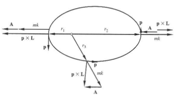
The LRL vector is used to describe shapes of orbits in two body central force problems. In the figure above, the LRL vector is described by \(\vec{p}\), \(L\), constant \(mk\), and \(e\). Respectively, the linear momentum, angular momentum, magnitude factor, and eccentricity. Vector \(\vec{A}\) always points in the same direction with the same magnitude \(mke\).
Another thing to note is that \(\vec{A}\) is a conserved vector.
Consider a central force described by: \(f(r) = - \frac{k}{r^{2}}\)
Vectorially, for a general central force, Newton’s second law can be written as:
\[\dot{\vec{p}} = f(r) \frac{\vec{r}}{r}\]with \(\vec{p} = m \dot{\vec{r}}\).
Evaluating the cross product of \(\dot{\vec{p}}\) with angular momentum \(\vec{L}\) (recall \(\vec{L} = \vec{r} \times \vec{p}\) )…
\[\dot{\vec{p}} \times \vec{L} = \dot{\vec{p}} \times (\vec{r} \times \vec{p} ) = f(r) \frac{\vec{r}}{r} \times ( \vec{r} \times \vec{p} ) = \frac{m f(r)}{r} \vec{r} \times ( r \times \dot{\vec{r}} )\]To deal with the triple product, we take advantage of umm… an “approximation” namely:
\[\vec{a} \times ( \vec{b} \times \vec{c} ) = \vec{b} ( \vec{a} \dot{} \vec{c} ) - \vec{c} ( \vec{a} \dot{} \vec{b} )\]It should be noted that this approach to triple cross products only works with vectors. This would be castostrophic if applied to operators!
\[\dot{\vec{p}} \times \vec{L} = m \frac{f(r)}{r} \bigg[ \vec{r} ( \vec{r} \dot{} \dot{\vec{r}} ) - \dot{\vec{r}} ( \vec{r} \dot{} \vec{r} ) \bigg]\]At this point, it might seem like we are losing vector information somehow. However, note that the velocity vector has two components ( \(v_{\bot}\) and \(v_{\parallel}\)) and it turns out that we only keep the parallel components of the vector.
\[\frac{d}{dt} \bigg[ \vec{p} \times \vec{L} \bigg] = \dot{\vec{p}} \times \vec{L} + \vec{p} \times \dot{\vec{L}}\] \[= m \frac{f(\vec{r}}{r} \bigg[ \vec{r} ( \vec{r} \dot{} \dot{\vec{r}} ) - \dot{\vec{r}} \dot{} r^{2} \bigg]\]Using \(\vec{r} \dot{} \dot{\vec{r}} = \frac{1}{2} \frac{d}{dt} ( \vec{r} \dot{} \vec{r} ) = r \dot{r}\), the equation is further simplified to:
\[\frac{d}{dt} \big[ \vec{p} \times \vec{L} \big] = -m f(r) r^{2} \bigg[ \frac{d}{dt} \bigg( \frac{\vec{r}}{r} \bigg) \bigg]\] \[\frac{d}{dt} \big[ \vec{p} \times \vec{L} \big] = \frac{d}{dt} \bigg( \frac{mkr}{r}\bigg)\]Notice that the right hand side of the equation does not have time , \(t\), as an explicit variable. This states that for the Kepler problem, there exists a conserved vector, that we’ll call \(\vec{A}\). Otherwise known as the Lagrange-Runge-Lenz Vector:
\[\vec{A} = \vec{p} \times \vec{L} - mk \frac{\vec{r}}{r}\]Let’s evaluate \(\vec{A} \dot{} \vec{L}\). \(L\) is perpendicular to \(\vec{p} \times \vec{L}\) and \(r\) is perpendicular to \(\vec{L} = \vec{r} \times \vec{p}\). What this means is that \(\vec{A}\) is always in the plane of the orbit. Mathematically:
\[\vec{A} \dot{} \vec{L} = ( \vec{p} \times \vec{L} - mk \frac{\vec{r}}{r} ) \dot{} \vec{L} = (\vec{p} \times \vec{L} ) \dot{} \vec{L} - \frac{mk}{r} \vec{r} \dot{} \vec{L} = 0\]Let \(\theta\) be the angle between \(\vec{r}\) and the fixed direction of \(\vec{A}\), the dot product between them comes out to be:
\[\vec{A} \times \vec{r} = Ar \cos(\theta) = \vec{r} \dot{} (\vec{p} \times \vec{L} ) - mkr\]Taking a closer look at \(\vec{r} \dot{} (\vec{p} \times \vec{L} )\), we can obtain a simplified form by cycling the product:
\[\vec{r} \dot{} (\vec{p} \times \vec{L} ) = - \vec{p} ( \vec{L} \times \vec{r} ) = \vec{L} \dot{} (\vec{r} \times \vec{p} ) = \vec{L} \dot{} \vec{L} = l^{2}\]Showing that the dot product between the two vectors is:
\[Ar \cos(\theta) = l^{2} - mkr\]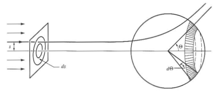
Some things to note from the figure above:
First we introduce some differential angle \(d \Omega\):
\[d\Omega = 2\pi h d\Theta\]Let \(h\) be the distance between the axis and height of the sphere’s radius that points from the central force. \(h\) can be defined as:
\[h = R \sin(\Theta)\]Applying \(R = 1\), \(h\) simplifies to \(h = \sin(\theta)\)
\[d\Omega = 2\pi \sin(\Theta) d\Theta\]Introducing some more variables:
Vectorially, \(\vec{r} = \vec{s} + \vec{r}_{0}\).
Using the definition of angular momentum:
\[\vec{L} = \vec{r} \times \vec{p}_{0} = ( \vec{r}_{0} + \vec{s} ) \times \vec{p}_{0} = \vec{r}_{0} \times \vec{p}_{0} + \vec{s} \times \vec{p}_{0}\]Since \(\vec{r}_{0} \parallel \vec{p}_{0}\) the cross product between them is \(0\) so we are left with:
\[\vec{L} = \vec{s} \times \vec{p}_{0}\]Now recall that in central force problems we can do away with vector information without loss of generality, the magnitude of angular momentum is:
\[| \vec{L} | = l = s p_{0} = s v_{0} m\]Using conservation of energy where \(E = \frac{1}{2} m v^{2}_{0}\), solve for \(v_{0}\) and substitute into \(l\) equation:
\[l = s \sqrt{2Em}\]This shows that the scattering angle is determined by impact parameter and energy!
The scattering cross section for a given angle is defined as:
\[\sigma (\vec{\Omega}) d \Omega = \frac{dN_{s}}{I}\]In English, the total scattering cross section is the ratio between the number of particles scattered into solid angle \(d\Omega\) per unit time (\(dN_{s}\)) versus incident intensity \(I\).
Using the previously defined solid angle, we can substitute a few term:
\[I \sigma (\Theta) 2 \pi \sin(\Theta) |d \Theta | = dN_{s}\]Note the absolute value sign on \(d \Theta\). Negative angles are possible, but of course, the number of particles cannot be negative. It should also be stated that \(dN_{s} ( \Theta, \Theta + d\Theta)\).
At the incident end, the impact parameter \(s\) traces out a ring \(ds\). The number of incident particles can be written as:
\[dN_{i} = I (area\; of\;ring)\] \[= I 2 \pi s |ds|\]Demanding the conservation of particles, the number of incident partcles must equal the number of scattered particles, \(dN_{i} = dN_{s}\). Combining the two equations yields:
\[I 2\pi s |ds| = I \sigma (\Theta) 2 \pi \sin(\Theta) |d \Theta |\]After some cancellation an solving for the scattering cross section, \(\sigma(\Theta)\):
\[\sigma(\Theta) = \frac{s}{\sin(\Theta)} \big| \frac{ds}{d\Theta} \big|\]This equation determines the probability of scattering at a certain angle.
Unfortunately, an equation for \(s(\Theta,E)\) does not exist at this point so, taking a closer look at the \(\frac{ds}{d\Theta}\) term, we can evaluate this using the orbital equation.
Using the figure above, the bounds of \(\vec{r}\) and \(\Psi\) are:
Using these bounds we can define the scattering angle, \(\Theta\) and the angle used in Kepler’s problem \(\theta\)
\[\Theta = \pi - 2\Psi_{m}\] \[\theta = \pi - \Psi\]Remembering that \(E\) is conservered:
\[E = \frac{1}{2} m \dot{r}^{2} + \frac{1}{2} \frac{l^{2}}{mr^{2}} + V(r)\] \[\dot{r} = \bigg[ \frac{2}{m} (E - V(r) ) - \frac{1}{2} \frac{l^{2}}{mr^{2}} \bigg]^{1/2} = \frac{dr}{dt}\]Using the definition of anglular momentum in a central force:
\[l = mr^{2} \dot{\theta} = m r^{2} \frac{d\theta}{dt}\] \[dt = \frac{m r^{2}}{l} d\theta\]The integral with respect to \(dt\) is transformed in terms of \(d\theta\):
\[\int^{\theta}_{\theta_{0}} d\theta = \int^{r}_{-\infty} \frac{dr}{r^{2} \big[ \frac{2mE}{l^{2}} - \frac{2mV}{l^{2} } \big]^{1/2} }\](Recognize that this was the solution to Kepler’s problem!)
Recall that \(\theta = \pi - \Psi\), we can write this equation in terms of \(\Psi\), that is, \(-\Psi = \theta - \pi\). Using that, we can work on the integration bounds on the orbital equation:
\[\theta - \theta_{0} = \int^{r}_{-\infty} ...\] \[\theta - \pi = \int^{r}_{-\infty} ...\] \[\theta = \pi + \int^{r}_{-\infty} ...\] \[- \Psi = \int^{-\infty}_{r} ...\] \[\Psi = \int^{-\infty}_{r} ...\] \[- \Psi = \int^{-\infty}_{r} = \int^{-\infty}_{r} \frac{dr}{r^{2} \big[ \frac{2mE}{l^{2}} - \frac{2mV}{l^{2} - \frac{1}{r^{2}}} \big]^{1/2} }\]This gives us an equation for the maximum angle of \(\Psi\):
\[\Psi_{m} = \int^{-\infty}_{r} \frac{dr}{r^{2} \big[ \frac{2mE}{l^{2}} - \frac{2mV}{l^{2}} - \frac{1}{r^{2}} \big]^{1/2} }\]This can still be further worked on by \(\Theta\) in terms of \(s\).
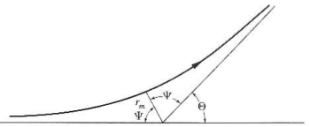 \(\Psi\) is defined as the angle between the incoming asymptote and the periapsis direction. \(\Psi\) can be obtained from the orbital equation by setting \(r_{0}\) when \(\theta_{0} = \pi\).
Since the orbit must be symmetric about the direction of the periapsis, the scattering anlge is defined:
\[\Theta = \pi - 2 \Psi_{m}\]Replacing \(\Psi_{m}\) with its definition gives:
\[\Theta = \pi - 2 \int^{-\infty}_{r} \frac{dr}{r^{2} \big[ \frac{2mE}{l^{2}} - \frac{2mV}{l^{2} } - \frac{1}{r^{2}} \big]^{1/2} }\]Using the relationship that \(r = \frac{1}{s^{2}}\):
\[\Theta = \pi - 2 \int^{-\infty}_{r} \frac{sdr}{r \big[ r^{2} - r^{2} \frac{V}{E} - s^{2} \big]^{1/2} }\]Rewriting the integral by way of u-substitution ( \(u = \frac{1}{r}\), \(dr = -\frac{1}{u^{2}} du\), \(r=\frac{1}{u}\) , \(du = -\frac{1}{r^{2}}dr\), when \(r \rightarrow \infty = 0\) and \(r \rightarrow r_{m} = u_{max}\) )
\[\Theta = \pi - 2 \int^{0}_{u_{max}} \frac{sdr}{ \big[ 1 - \frac{V}{E} - s^{2} u^{2} \big]^{1/2} }\]We have come to a place where we can choose the potential \(V\) in this master equation.
Consider the repulsive scattering of charged particles by a Coulomb Field. The force field of the two fixed charges \(-Ze\) and \(-Z' e\) can be written as:
\[f = \frac{Z Z' e^{2}}{r^{2}}\]where \(k = - Z Z' e^{2}\) so the force field takes the form of Kepler’s Problem \(f = \frac{k}{r}\).
For a repulsive interaction:
\[\frac{1}{r} = - \frac{mk}{l^{2}} \bigg[ \epsilon \cos(\theta - \theta') + 1 \bigg]\]With \(E>0\), the orbit is hyperbolic and the eccentricity is:
\[\epsilon = \sqrt{1 + \frac{2El^{2}}{mk^{2}}}\]Plugging in the definitions of \(k\) and \(l\) reduces \(\epsilon\) to:
\[\epsilon = \sqrt{ 1 + (\frac{2Es}{Z Z' e^{2}})^{2} }\]Replacing the term:
\[\frac{mk}{l^{2}} = \frac{1}{\alpha} = -\frac{m Z Z' e^{2}}{l^{2}}\]The equation for \(\frac{1}{r}\) becomes:
\[\frac{1}{r} = -\frac{m Z Z' e^{2}}{l^{2}} \bigg[ \epsilon \cos(\theta - \theta') + 1 \bigg]\]Remember that \(\theta'\) is the initial condition of the integration, in this case, \(\theta' = \pi\). So, \(\cos(\theta-\pi) = -\cos(\theta)\).
\[\frac{1}{r} = \frac{mk}{l^{2}} \bigg[ \epsilon \cos(\theta) - 1 \bigg]\]Refering to the diagram, at \(r_{min}\), the periapsis, we choose \(\cos(\theta)\) such that it is maximize, in other words, when \(\cos(\theta) = 1\).
Furthermore, \(r = 0\) as \(r \rightarrow - \infty\).
\[0 = \frac{mk}{l^{2}} \bigg[ \epsilon - 1 \bigg]\]In the direction of the incoming asymptote, \(\Psi_{m}\):
\[\cos(\Psi_{m}) = \frac{1}{\epsilon}\]Making use of \(\Theta = \pi = 2 \Psi_{m}\) we can derive some trigonometric terms for scattering.
\[\Psi_{m} = \frac{\pi}{2} - \frac{\Theta}{2} \rightarrow \cos(\frac{\pi}{2} - \frac{\Theta}{2}) = \sin(\frac{\Theta}{2})\]so the trigonometric relationship to the eccentricity can be written as:
\[\epsilon = \frac{1}{\cos(\Psi_{m})} = \frac{1}{\sin(\frac{\Theta}{2})}\]Using the \(\sin\) term, square both sides, introduce \(1\) by adding and subtracting it.
\[\epsilon^{2} = \frac{1}{\sin(\frac{\Theta}{2})} + 1 - 1\] \[\epsilon^{2} - 1= \frac{1}{\sin(\frac{\Theta}{2})} - \frac{\sin(\frac{\Theta}{2})}{\sin(\frac{\Theta}{2})}\] \[\epsilon^{2} - 1 = \cot^{2}(\frac{\Theta}{2})\]Reintroducing the definition of eccentricity gives a relationship:
\[\cot(\frac{\Theta}{2}) = \frac{2 s E}{Z Z' e^{2}}\]Now, we have an equation that expresses the impact parameter \(s\) as a function of the scattering angle \(\Theta\) and energy \(E\):
\[s = \frac{Z Z' e^{2}}{\sin(\Theta)} \cot \big(\frac{\Theta}{2}\big)\]Now that an equation for \(s(\Theta,E)\) has been obtained, the derivative in the scattering cross section equation can finally be evaluated!
\[\sigma(\Theta) = \frac{s}{\sin(\Theta)} \big| \frac{ds}{d\Theta} \big|\] \[\sigma(\Theta) = \frac{s}{\sin(\Theta)} \big[ \frac{Z Z'}{2E} \frac{1}{2} \cot^(\frac{\Theta}{2}) \big] \big[ \frac{Z Z' e^{2}}{2 E} \frac{1}{2} \csc^{2}(\frac{\Theta}{2}) \big] = \frac{1}{2} (\frac{Z Z' e^{2}}{2E})^{2} \frac{\cos(\frac{\Theta}{2}{2})}{\sin(\frac{\Theta}{2})} \frac{\csc^{2}(\frac{\Theta}{2})}{2\sin(\frac{\Theta}{2})\cos(\frac{\Theta}{2})}\]The equation for Rutherford Scattering is:
\[\sigma(\Theta) = \frac{1}{4} \bigg(\frac{Z Z' e^{2}}{2 E} \bigg)^{2} \csc^{4}\bigg(\frac{\Theta}{2} \bigg)\]A rigid body is defined as a system of mass points remaining at a constant distance of each other under the influence of holonomic constraints. The first question to ask is: How many independent coordinates are needed to describe the motion of a rigid body?
[insert a nice photo of a rigid body here?]
There are two coordinate systems to pay attention to: the standard \(x,y,z\) frame and the frame relative to the center of mass \(x',y',z'\). The goal is to establish a flow of information from \(\{ x, y, z\}\) to \(\{x',y',z'\}\).
Vector \(\vec{R}\) points from the origin to the center of mass and is described by the three coordinates:
\[\vec{R} = \hat{i} x + \hat{j} y + \hat{k} z\]along with 3 angles that determine the orientation.
The general mathematical procedure is to establish the system of reference:
1) Establish the system of reference:
\((x,y,z) +\) basis \((\hat{i}, \hat{j}, \hat{k})\)
2) Establish the basis that is fixed to the rotating body:
\((x',y',z') +\) basis \((\hat{i}', \hat{j}',\hat{k}')\)
The velocity and acceleration of \(\vec{R}\) can be written as
\[\frac{d\vec{R}}{dt} = \vec{V}\] \[\vec{A} = \frac{d\vec{R}^{2}}{dt^{2}}\]Turning the focus to rotation about the center of mass:
We choose some point \(p\) with \(\vec{r}\) pointing to it:
\[\vec{r}' = \hat{i} x' + \hat{j} y' + \hat{k} z'\]The question is: how do we get point \(p\) in the \((x,y,z)\) frame? If we know a vector, then we can determine its projections. In other words, taking \(x'\) as an example, it is simply a projection of \(\vec{r}'\) onto \(\hat{i}\)!
\[x' = \vec{r}' \dot{} \hat{i}' = (x' \hat{i}' + y' \hat{j}' + z' \hat{k}') \dot{} \hat{i}'\] \[= x' (\hat{i}' \dot{} \hat{i}) + y (\hat{j}' \dot{} \hat{i}) + z' (\hat{k}' \dot{} \hat{i})\]In terms of cosines:
\[= x' \cos(\theta_{11}) + y' (\cos(\theta_{21}) + z' \cos(\theta_{31})\]The same can be done for \(\vec{r}'\) dotted into \(\hat{j}\) and \(\hat{k}\):
\[\vec{r}' \dot{} \hat{j} \rightarrow \cos(\theta_{12}), \cos(\theta_{22}) , \cos(\theta_{32})\] \[\vec{r}' \dot{} \hat{k} \rightarrow \cos(\theta_{13}), \cos(\theta_{23}) , \cos(\theta_{33})\]Using this information, we can rewrite \(\vec{r}\):
\[\vec{r} = \vec{r}' = \hat{i} x + \hat{j} y + \hat{k} z = (\vec{r}' \dot{} \hat{i}) \dot{} \hat{i} + (\vec{r}' \dot{} \hat{j}) \dot{} \hat{j} + (\vec{r}' \dot{} \hat{k}) \hat{k}\]Essentially, the \(x'\) frame is projected onto \(x\) with the following relation:
\[x' = x \cos(\theta_{11}) + y \cos(\theta_{21}) + z \cos(\theta_{31})\]In total there are 12 parameters to keep track of, 3 translation and 9 angles.
To stay consistent with column vector notation, we change the notion of the \(x,y,z\) coordinates to:
\[x \rightarrow x_{1}\] \[y \rightarrow x_{2}\] \[z \rightarrow x_{3}\]where the column vector notation is:
\[\vec{x} = \begin{bmatrix} x_{1}\\ x_{2}\\ x_{3} \end{bmatrix}\]From here, the transformation matrix established. Starting from a system of equations with elements \(a_{ij}\):
\[x_{1} = a_{11} x_{1}' + a_{12} x_{2}' + a_{13} x_{3}'\] \[x_{2} = a_{21} x_{1}' + a_{22} x_{2}' + a_{23} x_{3}'\] \[x_{3} = a_{31} x_{1}' + a_{32} x_{2}' + a_{33} x_{3}'\]The corresponding matrix is:
\[\vec{A} = \begin{bmatrix} a_{11} & a_{12} & a_{13} \\ a_{21} & a_{22} & a_{23} \\ a_{31} & a_{32} & a_{33} \end{bmatrix}\]so the transformation equation is given by:
\[\vec{r}' = \vec{A} \vec{r}\]where a can be considered a matrix that “operates” on \(\vec{r}\).
Kronecker Delta
A common convention of concisely writing summations of orthogonality conditions:
\(a_{ij} a_{ik} = 1\) if \(j=k\)
\(a_{ij} a_{ik} = 0\) if \(j \neq k\)
More compactly,
\(a_{ij} a_{ik} = \delta_{jk}\) with \(j,k = 1,2,3\)
Recall that a rigid body can be described by 6 degrees of freedom: 3 translational and 3 rotational. Consider rotation a vector \(\v{b}\) to its new position \(\v{b}'\) by some angle \(\phi\).
The rotation can be expressed by matricies as:
\[\begin{bmatrix} b'_{x} \\ b'_{y} \end{bmatrix} = \begin{bmatrix} \cos\phi & \sin\phi \\ -\sin\phi & \cos\phi \end{bmatrix} \begin{bmatrix} b_{x} \\ b_{y} \end{bmatrix}\]Where \(A_{ij} = \begin{bmatrix} \cos\phi & \sin\phi \\ -\sin\phi & \cos\phi \end{bmatrix}\) is the standard rotation matrix for in 2 dimensions.
\(a\) is the rotation axis and \(\theta\) is the rotation angle.
The rotation matrix is orthogonal, so by definition \(\v{A}^{T} \v{A} = \v{1}\), or:
\[\v{A}_{a,\theta}^{T} = \v{A}_{a,\theta}^{-1}\] \[det(\v{A_{a,\theta}}) = 1\] \[\v{A}_{a,(\theta + r)} = \v{A}_{a,\theta} \dot{} \v{A}_{a,r}\] \[\v{A}_{a,0} = \v{I}\]We can express successive rotations through matrix multiplication:
\[\vec{A} = \begin{bmatrix} -1 & 0 & 0 \\ 0 & -1 & 0 \\ 0 & 0 & 1 \end{bmatrix} \begin{bmatrix} 1 & 0 & 0 \\ 0 & 1 & 0 \\ 0 & 0 & -1 \end{bmatrix} = \begin{bmatrix} -1 & 0 & 0 \\ 0 & -1 & 0 \\ 0 & 0 & -1 \end{bmatrix}\]Physically, the successive multiplication of these matricies is essentially:
(rotation about \(180\circ\) about \(z\))(reflection in the \(xy\) plane) = inversion
The inversion matrix is defined as:
\[\vec{A} = \begin{vmatrix} -1 & 0 & 0 \\ 0 & -1 & 0 \\ 0 & 0 & -1 \end{vmatrix} = -1\]If \(\lvert A \rvert = +1\), then it is a proper rotation.
If \(\lvert A \rvert = -1\), then it is an improper rotation, and cannot achieve continuous rotations.
Goldstein describes Euler’s theorem as:
“A general displacement of a rigid body with one point fixed is a rotation about an axis”
In the context of matricies, Euler’s theorem can be restated as:
“The real orthogonal matrix specifying the physical motion of a rigid body with one point fixed always has the eigenvalue +1”
For example, a matrix that takes the form:
\[\begin{bmatrix} \cos\phi & \sin\phi & 0 \\ -\sin\phi & \cos\phi & 0 \\ 0 & 0 & 1 \end{bmatrix}\]This matrix represents a rotation about the \(z\) axis.
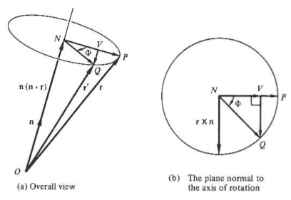
Consider a clockwise rotation of a vector about an axis. The initial vector \(\vec{r}\) is denoted \(\vec{OP}\) and the final position shown as \(\vec{r}'\) is denoted as \(\vec{OQ}\). The axis of rotation is about unit vector \(\hat{n}\).
From the figures above, some vector definitions can be written down. First order of business is to write down \(\v{r}'\) in terms of \(\vec{r}, \phi, \h{n}\).
\(\v{r}'\) is just a some of a three easily identifiable vectors:
\[\v{r}' = \v{ON} + \v{NV} + \v{VQ}\]We can redefine some of these vectors into more useful terms:
\(\vec{ON}\) is a projection of \(\vec{r}\) onto \(\hat{n}\) and can be written as \(\hat{n}(\hat{n} \dot{} \vec{r})\).
Vector \(\vec{NP}\) can be written as \(\vec{r} - \vec{n}(\hat{n} \dot{} \vec{r})\) with the same magnitude of \(\vec{NQ}\) and \(\vec{r} \times \hat{n}\).
Notice that \(\lvert \vec{NQ} \rvert = \lvert \vec{NP} \rvert\), which can be substituted for the definition of \(\abs \v{NV} \abs\):
\[\abs \v{NV} \abs = \abs \v{NQ} \abs \cos\phi = \abs \v{NP} \abs \cos\phi = [\v{r} - \h{n} (\v{r} \d \h{n})] \cos\phi\]Matricies can be expanded as a sum over their element indicies:
\[(\v{A} (\v{B} \v{C}))_{ij} = \sum_{k} a_{ik} (\v{B} \v{C})_kj = \sum_{k} a_{ik} \sum_{l} b_{kl} c_{lj} = \sum_{k} \sum_{l} a_{ik} b_{kl} c_{lj} = \sum_{l} (\v{A} \v{B})_{il} c_{lj} = ((\v{A} \v{B}) C)_{ij}\]Also, for free, this shows that matrix multiplication is associative.
An orthogonal matrix is a real square matrix whose columns and rows are orthonomal vectors. By definition:
\[\v{A} \v{\~{A}} = \v{\~{A}} \v{A} = \v{1}\]Also, a matrix is orthogonal if its transpose is equal to its inverse:
\[\v{\~{A}} = \v{A}^{-1}\]A symmetric matrix is simply a real square matrix that is equal to its transpose. Mathematically, \(\v{A}^{T} = \v{A}\). For example:
\[\begin{bmatrix} 1 & 1 & -1 \\ 1 & 2 & 0 \\ -1 & 0 & 0 \\ \end{bmatrix}\]Recall that the diagonals and off diagonals of \(\vec{I}_{jk}\) can be obtained with:
\[\vec{I}_{jk} = \int_{V} \rho(\vec{r}) (r^{2} \delta_{jk} - x_{j} x_{k}) dV\]\(\vec{I}\) is classified as a tensor, more specifically, a tensor of the second rank.
The diagonals in the matrix elements is given by:
\[\vec{I}_{xx} = \int_{V} \rho(\vec{r}) (r^{2} - x^{2}) dV\]In the standard three dimensional cartesian space, a Tensor of the \(N\)th rank may be defined as:
\(\vec{T}_{ijk...}\) (with \(N\) indicies)
In English, a tensor of rank \(N\) has \(3^{N}\) components and \(N\) indicies,
that can transform under an orthoganal transformation of coodintes, \(A\) according to the following scheme:
\[\vec{T}'_{ijk}...(\v{x}') = a_{il} a_{jm} a_{kn}... T_{lmn}...(\vec{x})\]In other words, a tensor with one component is a tensor of zero ranks, invariant under orthogonal transfomrations.
A tensor of first rank can be written as: \(T_{i}' = a_{ij} T{j}\)
which is equivalent to a vector.
Two vectors, call them \(\v{A}\) and \(\v{B}\), can be used to construct a second rank tensor. \(\v{A}\) and \(\v{B}\) have components \(A_{i}\), \(B_{i}\).
Let \(\v{T}\) be a second rank tensor. Then,
\[\v{T}_{ij} = \v{A}_{i} \v{B}_{j}\]deconstructed…
\[\v{T} = \begin{bmatrix} \v{T}_{xx} & \v{T}_{xy} \\ \v{T}_{yx} & \v{T}_{yy} \end{bmatrix} = \begin{bmatrix} \v{A}_{x} \v{B}_{x} & \v{A}_{x} \v{B}_{y} \\ \v{A}_{y} \v{B}_{x} & \v{A}_{y} \v{B}_{y} \end{bmatrix}\]Each component in the tensor should transform in the scheme mentioned above as:
\[\v{T}'_{xy} = \sum_{i=1}^{3} \sum_{j=1}^{3} a_{xi} a_{yj} T_{ij} = a_{xi} a_{yj} A_{i} B_{j} = a_{ai} A_{i} a_{ay} B_{j} = A'_{x} B'_{y}\]A unit tensor, denoted \(\v{1}\) has components:
\[\v{1}_{ij} = \delta_{ij}\]where \(\delta_{ij}\) is the kronecker delta, \(\delta_{ij} = 1\) if \(i=j\).
Classical Mechanics by Goldstein, Poole & Safko
Mechanics by Landau & Lifshitz